Linear Algebra

Lists : A list of length 𝑛 is an ordered collection of 𝑛 elements. Two lists are equal if and only if they have the same length and the same elements in the same order.

A vector space $V$ over the field $\mathbb{R}$ is a set of vectors together with two operations:

• Vector addition : $+:V\times V\to V$ Add two vectors to get another vector.
• Scalar multiplication $\cdot :\mathbb{R}\times V\to V$ Multiply a vector by a real number (scalar).

Elements of a vector space are called vectors or points.

Depending on the vector space, a vector could be:

• A column of numbers: $\left(\begin{array}{c}1\\ 2\\ 3\end{array}\right)$

• A matrix: $\left(\begin{array}{cc}1& 2\\ 3& 4\end{array}\right)$

• A polynomial: $1+2x+3x^2$

• A function:$f(x)=\sin x$

---

The projection of point $x$ onto direction $w$. $w^{T}x$

• $x$ = The vector being analyzed (column vector)
• $w$ = The direction or weight vector (column vector)
• $w^T$ = A row vector acting on $x$

Even though the dot product is numerically symmetric: $w^{T}x=x^{T}w$ Writing it as $w^{T}x$ keeps semantic roles consistent across fields : In Machine Learning & Statistics

• $x$ = The data / input (the object being observed)
• $w$ = The parameter / direction / filter / weight In Geometry
• $x$ = The vector being decomposed
• $w$ = The reference direction

---

Subspace

A subspace of a vector space $V$ is a subset $S\subseteq V$ that is itself a vector space under the same operations. It must satisfy three conditions:

1. Contains the origin: $0\in S$
2. Closed under addition: if $\mathbf{u},\mathbf{v}\in S$, then $\mathbf{u}+\mathbf{v}\in S$
3. Closed under scalar multiplication: if $\mathbf{v}\in S$ and $c\in \mathbb{R}$, then $c\mathbf{v}\in S$

Examples

• In ${\mathbb{R}}^3$: any line or plane through the origin is a subspace
• In ${\mathbb{R}}^3$: a plane not through the origin is not a subspace

A subspace always passes through the origin. If it doesn’t, it is called an affine subspace.

An affine subspace is a shifted (translated) version of a subspace. It has the form:

$S+{\mathbf{v}}_0=\mathbf{s}+{\mathbf{v}}_0\mid \mathbf{s}\in S$

where $S$ is a subspace and ${\mathbf{v}}_0$ is a fixed offset vector.

---

Hyperplane

A hyperplane is a flat geometric object of dimension $n-1$ inside an $n$-dimensional space. It is the most natural way to “cut” a space into two parts with a single boundary.

Normal Form ($H_1$): A normal form describes a geometric object using a vector that is **perpendicular to it.

A hyperplane in ${\mathbb{R}}^n$ can be defined in normal form as:

$H=\{x\in {\mathbb{R}}^n:{\omega }^{T}x=\alpha \}$ (Set definition)

• $x\in {\mathbb{R}}^n$ → point in n-dimensional space
• $\omega \in {\mathbb{R}}^n$ → normal vector (weight vector)
• $\alpha \in \mathbb{R}$ → offset (bias term)

Linear Equation Form A hyperplane is the set of all points $\mathbf{x}\in {\mathbb{R}}^n$ satisfying a single linear equation:

$a_1{x}_1+a_2{x}_2+\cdots +a_n{x}_n=b$

or in vector form:

$\mathbf{w}\cdot \mathbf{x}=b$

where:

• $\mathbf{w}=(a_1,a_2,\dots ,a_n)\ne 0$ is the normal vector
• $b\in \mathbb{R}$ is a scalar constant
• $\mathbf{x}\in {\mathbb{R}}^n$ is any point on the hyperplane

The set:

${\omega }^{T}x=\alpha$

describes all points whose projection onto $\omega$ is constant.

• all points in $H$ share the same dot product with $\omega$
• they lie on a flat $(n-1)$-dimensional surface
• $\omega$ determines orientation
• $\alpha$ determines shift (offset from origin)
• changing $\omega$ rotates the hyperplane
• changing $\alpha$ translates it

If $\alpha =0$, then:

${\omega }^{T}x=0$

This hyperplane passes through the origin.

A hyperplane in ${\mathbb{R}}^n$ is defined by ${\omega }^{T}x=\alpha$, where $\omega$ is the normal vector perpendicular to the $(n-1)$-dimensional surface.

Space	Hyperplane
${\mathbb{R}}^2$	Line
${\mathbb{R}}^3$	Plane
${\mathbb{R}}^n$	$(n-1)$-dimensional flat surface

Dividing space into two half-spaces :

A hyperplane splits ${\mathbb{R}}^n$ into exactly two half-spaces:

$H^{+}=\mathbf{x}\mid \mathbf{w}\cdot \mathbf{x}>b$ $H^{-}=\mathbf{x}\mid \mathbf{w}\cdot \mathbf{x}<b$

“half-space” means two separated regions — it does not imply equal volume or measure.

Point-Directional Form ($H_2$): Instead of a perpendicular line, you define the boundary by picking a starting point $y_0$ that sits on the boundary, and then spanning out in $n-1$ different directions using linearly independent vectors $y_1,...,y_{n-1}$. Independent direction vectors are linearly independent vectors lying inside the hyperplane that span all possible directions within it.

• $x=y_0+{\sum }_{i=1}^{n-1}{\lambda }_i{y}_i$ means that any point $x$ on this boundary can be reached by starting at $y_0$ and moving along those direction vectors by some scaling factors ${\lambda }_i$.

Moving from $H_1$ to $H_2$ The primary goal of a linear classifier like a perceptron is to look at a new data point $x$ and decide which side of the boundary it falls on.

• Using $H_1$ (Normal Form): You only have to calculate a single dot product: $w^{T}x$. If the result is positive, it belongs to one class; if negative, the other. This is incredibly fast for a computer to process.
• Using $H_2$ (Point-Directional Form): To figure out which side of the boundary a point is on, you would have to solve a complex system of linear equations to find all the ${\lambda }_i$ scaling factors for every single data point. That would be computational.

---

Convex Set

A set $C\subseteq {\mathbb{R}}^n$ is convex if for any two points in the set, the entire line segment connecting them also lies in the set.

Formally, $C$ is convex if:

$\forall ,\mathbf{x},\mathbf{y}\in C,\forall ,\lambda \in [0,1]:\lambda \mathbf{x}+(1-\lambda )\mathbf{y}\in C$

The expression $\lambda \mathbf{x}+(1-\lambda )\mathbf{y}$ is called a convex combination of $\mathbf{x}$ and $\mathbf{y}$. As $\lambda$ varies from $0$ to $1$, it traces the straight line segment from $\mathbf{y}$ to $\mathbf{x}$. The formula $\lambda x+(1-\lambda )y$ is just the algebraic way to write “a straight line segment between $x$ and $y$

Intuition

A set is convex if you can “see” every point from every other point without leaving the set — no dents, holes, or concavities.

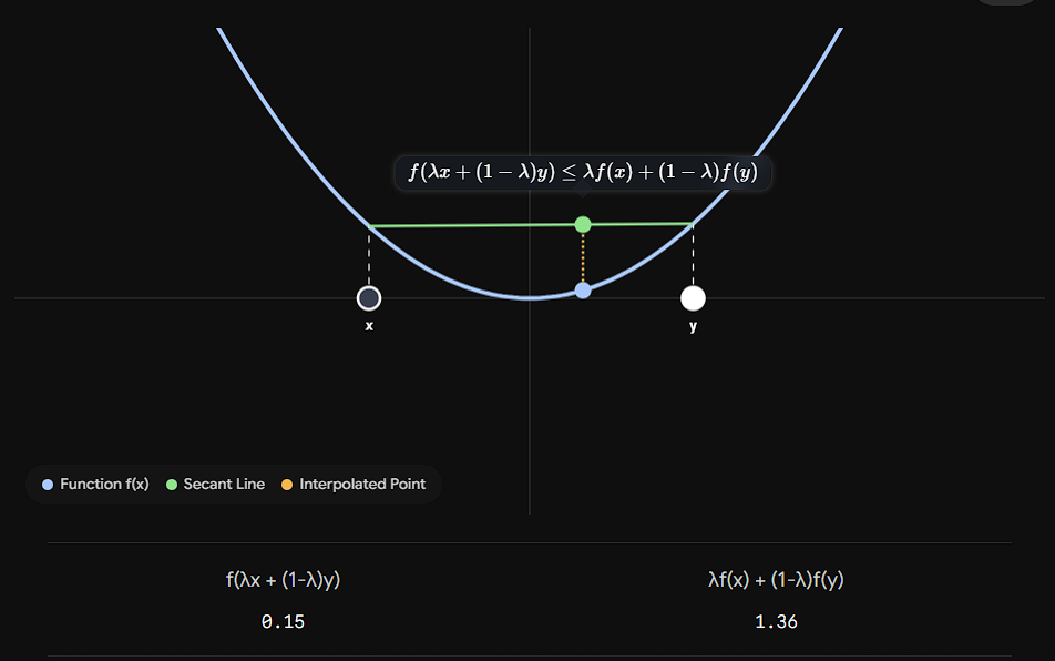
The function $f$ is convex if and only if the line segment connecting any two points on its graph lies above or on the graph itself. A function is convex if it is shaped like a right-side-up bowl : if you pick two points on the curve and draw a straight line (a secant line) between them, the actual curve of the function must sag below (or equal to) that straight line.

Jensen’s Inequality base :
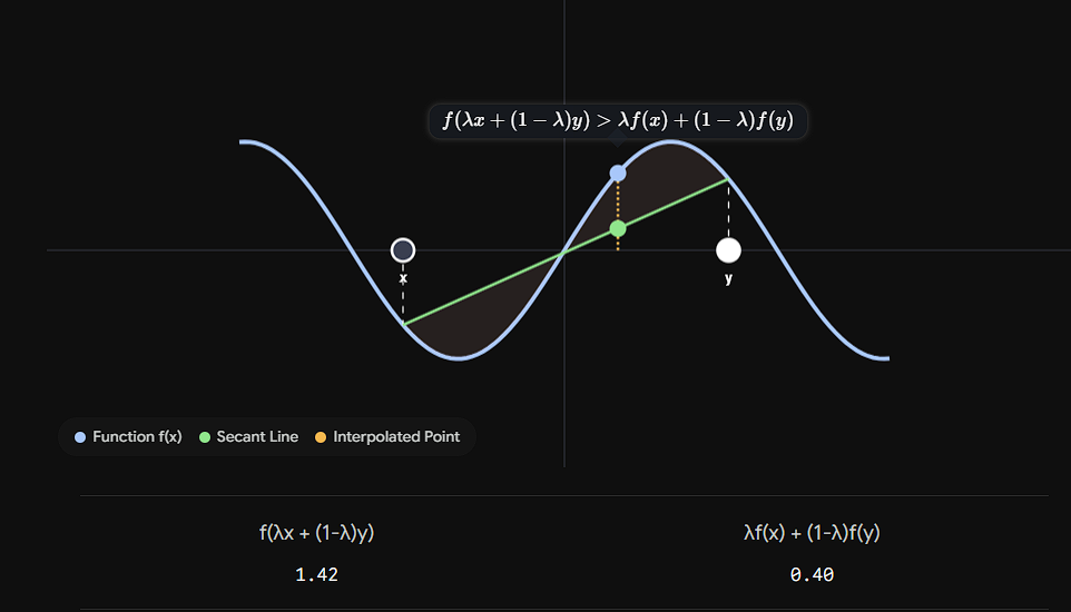
Let $f:M\to \mathbb{R}$ where the domain $M$ is a convex set, For any $x,y\in M$ and any $\lambda \in [0,1]$:

$f(\lambda x+(1-\lambda )y)\le \lambda f(x)+(1-\lambda )f(y)$

Non convex :

---

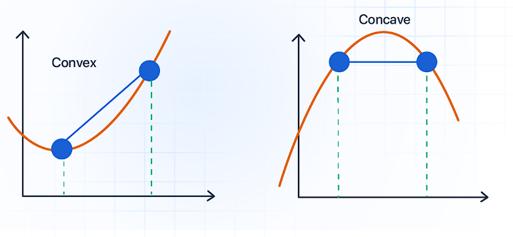
Linear functions are both convex and concave

Linearity ⇒ Both Convex and Concave

Consider the affine function:

$f(x)=c^{T}x+b$

A function is convex if for all $x,y$ and $\theta \in [0,1]$:

$f(\theta x+(1-\theta )y)\le \theta f(x)+(1-\theta )f(y)$

LHS : $f(\theta x+(1-\theta )y)$ $=c^T(\theta x+(1-\theta )y)+b$ $=\theta c^{T}x+(1-\theta )c^{T}y+b$

RHS : $\theta f(x)+(1-\theta )f(y)$ $=\theta (c^{T}x+b)+(1-\theta )(c^{T}y+b)$ $=\theta c^{T}x+(1-\theta )c^{T}y+\theta b+(1-\theta )b$ $=\theta c^{T}x+(1-\theta )c^{T}y+b$

$f(\theta x+(1-\theta )y)=\theta f(x)+(1-\theta )f(y)$

The function is:

• convex
• concave

linear/affine functions commute with convex combinations, so they induce zero curvature and generate convex (and concave) structure simultaneously.

---

Half-spaces

A half-space is one side of a hyperplane in an n-dimensional space.

Formally, a (closed) half-space is:

$H=x\in {\mathbb{R}}^n\mid a^{\top }x\le b$

where:

• $a\in {\mathbb{R}}^n$, $a\ne 0$
• $b\in \mathbb{R}$

The hyperplane boundary is:

$a^{\top }x=b$

• it has a flat boundary (hyperplane)
• it does not curve inward or outward
• it splits space into exactly two parts

There is also the open half-space:

$x\mid a^{\top }x<b$

Half-spaces are always convex sets.

A half-space is defined as:

$H^{+}=\mathbf{x}\in {\mathbb{R}}^n\mid \mathbf{w}\cdot \mathbf{x}\ge b$ ($H^{+}$ = Positive class region)

(The argument works identically for $H^{-}=\mathbf{x}\mid \mathbf{w}\cdot \mathbf{x}\le b$.)

Proof

Take any two points $\mathbf{x},\mathbf{y}\in H^{+}$. By definition:

$\mathbf{w}\cdot \mathbf{x}\ge b\text{and}\mathbf{w}\cdot \mathbf{y}\ge b$

Now take any convex combination $\mathbf{z}=\lambda \mathbf{x}+(1-\lambda )\mathbf{y}$ with $\lambda \in [0,1]$. We need to show $\mathbf{z}\in H^{+}$, i.e., $\mathbf{w}\cdot \mathbf{z}\ge b$.

$\mathbf{w}\cdot \mathbf{z}=\mathbf{w}\cdot (\lambda \mathbf{x}+(1-\lambda )\mathbf{y})$ $=\lambda (\mathbf{w}\cdot \mathbf{x})+(1-\lambda )(\mathbf{w}\cdot \mathbf{y})$

Since $\mathbf{w}\cdot \mathbf{x}\ge b$ and $\mathbf{w}\cdot \mathbf{y}\ge b$, and $\lambda \ge 0$, $(1-\lambda )\ge 0$, $\lambda +(1-\lambda )=1$:

$\ge \lambda b+(1-\lambda )b=b$

Therefore $\mathbf{w}\cdot \mathbf{z}\ge b$, so $\mathbf{z}\in H^{+}$.

The proof works because the dot product $f(\mathbf{x})=\mathbf{w}\cdot \mathbf{x}$ is a linear function, and linear functions preserve convex combinations:

$f(\lambda \mathbf{x}+(1-\lambda )\mathbf{y})=\lambda f(\mathbf{x})+(1-\lambda )f(\mathbf{y})$

A half-space is just the sublevel (or superlevel) set of a linear function and sublevel sets of linear (and more generally, convex) functions are always convex. If two points satisfy a linear inequality, every convex combination also satisfies it

Any convex polyhedron = intersection of finitely many half-spaces

---

A hyperplane $\mathbf{w}\cdot \mathbf{x}=b$ can be written as:

$\mathbf{x}\mid \mathbf{w}\cdot \mathbf{x}\ge b\cap \mathbf{x}\mid \mathbf{w}\cdot \mathbf{x}\le b$

Since both half-spaces are convex, and the intersection of convex sets is always convex, a hyperplane is also convex.

The intersection of any collection of convex sets is convex.

Any region defined by a finite number of linear inequalities (a polyhedron) is convex, since it is an intersection of half-spaces.

Any convex set can be written as the intersection of (possibly infinitely many) half-spaces.

A fundamental structural result in convex geometry states:

$C={\bigcap }_{\alpha \in A}\{x:a_{\alpha }^{T}x\le b_{\alpha }\}$

Each constraint: $a_{\alpha }^{T}x\le b_{\alpha }$ defines a half-space, i.e. one side of a hyperplane.

(a) Polyhedron (finite case)

If $A$ is finite:

$C=\{x:Ax\le b\}$

This is a polyhedron. A convex polyhedron is mathematically defined as the intersection of a finite number of half-spaces.

(b) Euclidean ball (infinite case)

A ball: $\Vert x{\Vert }_2\le r$ intersection of all tangent half-spaces.

Convex sets are exactly those regions that can be described entirely by linear inequalities.

---

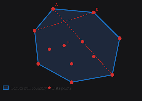
Convex Hull The convex hull is the smallest convex shape that encloses all points.

---

Norm A norm is a function $\Vert \cdot \Vert :V\to [0,\infty )$ such that the following hold for all $\lambda \in \mathbb{R}$ and $u,v\in V$:

• (i) Positivity: $\Vert v\Vert =0$ if and only if $v=0$.
• (ii) Homogeneity: $\Vert \lambda u\Vert =|\lambda |\Vert u\Vert$.
• (iii) Triangle inequality: $\Vert u+v\Vert \le \Vert u\Vert +\Vert v\Vert$.

We call the tuple $(V,\Vert \cdot \Vert )$ a normed space.

$\text{Norm}=\text{length of a vector}$

Common norms

${\ell }_p$ Norms

For $p\in [1,\infty )$, we denote:

$\Vert v\Vert {}_p={\left({\sum }_{i=1}^d|v_i|{}^p\right)}^{1/p}$

For $p=\infty$, we denote:

$\Vert v\Vert {}_{\infty }={\max }_{i=1,\dots ,d}|v_i|$

The ${\ell }_1$ Norm ($p=1$)

• Manhattan Distance or Taxicab Norm.
  • A way of measuring distance where you can only move along grid lines. In a city with a grid layout (like Manhattan), you can’t cut diagonally through buildings. You have to go along the streets, some blocks east/west, some blocks north/south.
• $\Vert v\Vert {}_1=|v_1|+|v_2|+\cdots +|v_d|$ (the sum of absolute values).
• Sparsity / Feature Selection (Lasso Regularization): In machine learning, using an ${\ell }_1$ penalty forces unimportant model weights to become exactly zero. This effectively selects the most important features.
• Robustness to Outliers: ${\ell }_1$ loss (Mean Absolute Error) is less sensitive to extreme outliers than ${\ell }_2$ loss.

The ${\ell }_2$ Norm ($p=2$)

• Euclidean Distance.
• $\Vert v\Vert {}_2=\sqrt{v_1^2+v_2^2+\cdots +v_d^2}$.
• Used for:
  • Weight Decay (Ridge Regularization / L2): In machine learning, it penalizes large weights to prevent overfitting, keeping the model stable and smooth.
  • Optimization (Mean Squared Error): Most machine learning optimization algorithms prefer ${\ell }_2$ because its derivative is mathematically clean and continuous everywhere.

The ${\ell }_{\infty }$ Norm ($p=\infty$)

• Chebyshev Distance or Maximum Norm.
• $\Vert v\Vert {}_{\infty }=\max (|v_1|,|v_2|,\dots ,|v_d|)$.
• Used for :
  • Adversarial Machine Learning: Often used to define a “budget” for an attacker trying to fool a model (e.g., “you can change any pixel in this image, but no single pixel can change by more than $ϵ$”).
  • Worst-case Analysis: It helps evaluate systems where you only care about the single largest error or deviation.

Example : Let $V={\mathbb{R}}^2$, and:

$v=\left(\begin{array}{c}3\\ 4\end{array}\right)\in V$

• ${\ell }_1$ norm (Manhattan distance):$\Vert v\Vert {}_1=|3|+|4|=7$

• ${\ell }_2$ norm (Ordinary Euclidean length):$\Vert v\Vert {}_2=\sqrt{3^2+4^2}=5$

• ${\ell }_{\infty }$ norm (Maximum/Chebyshev norm):
  $\Vert v\Vert {}_{\infty }=\max (|3|,|4|)=4$

The exact same vector has different “lengths” depending entirely on the norm you choose to measure it with.

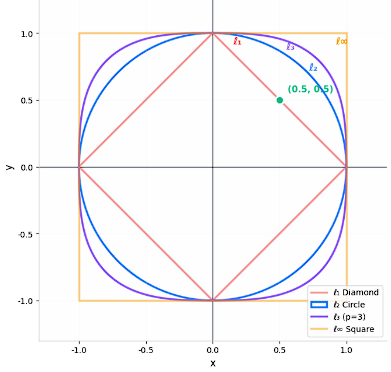
Example : A unit circle is defined as the set of all points that are exactly a distance of $1$ away from the origin $(0,0)$.

$\{v\in {\mathbb{R}}^2\mid \Vert v\Vert =1\}$

Because the norm $\Vert \cdot \Vert$ is how we measure “distance,” changing the norm fundamentally changes what points are considered “1 unit away” from the center.

• Under the ${\ell }_2$ norm, a unit circle is a perfect standard circle.
• Under the ${\ell }_1$ norm, a unit circle looks like a tilted diamond.
• Under the ${\ell }_{\infty }$ norm, a unit circle is a square.

Matrix Norms

Consider the space of $n\times m$ matrices, that is, ${\mathbb{R}}^{n\times m}$. Every matrix $A\in {\mathbb{R}}^{n\times m}$ can be identified with a linear function via

$(Av{)}_i={\sum }_{j=1}^m{A}_{i,j}{v}_j,i=1,\dots ,n.$

The following norms are frequently used on ${\mathbb{R}}^{n\times m}$:

• Frobenius norm: Measures the overall size of a matrix. $\Vert A\Vert {}_F=\sqrt{{\sum }_{i,j}|A_{i,j}|{}^2}$ $A=\left(\begin{array}{cc}1& 2\\ 3& 4\end{array}\right)$

$\Vert A\Vert {}_F=\sqrt{1^2+2^2+3^2+4^2}=\sqrt{30}$

A matrix is a function that transforms vectors: $A:{\mathbb{R}}^m\to {\mathbb{R}}^n$ It takes an input vector $v$ and produces: $Av$

• Induced norms: For every pair of norms $\Vert \cdot \Vert {}_a$ on ${\mathbb{R}}^m$ and $\Vert \cdot \Vert {}_b$ on ${\mathbb{R}}^n$, we can define the induced norm:

  $\Vert A\Vert {}_{a,b}:={\sup }_{\Vert v\Vert {}_a\le 1}\Vert Av\Vert {}_b={\sup }_{v\ne 0}\frac{\Vert Av\Vert {}_b}{\Vert v\Vert {}_a}$

  An induced norm measures the maximum possible “stretching factor” that the matrix $A$ can apply to any vector $v$.

$\Vert Av\Vert {}_b\le \Vert A\Vert {}_{a,b}\Vert v\Vert {}_a$

• Common Matrix Norms

  • Maximum absolute column sum ($1$-norm): Take the largest absolute column sum.
    $\Vert A\Vert {}_1={\max }_j{\sum }_i|A_{i,j}|$
  • Maximum absolute row sum ($\infty$-norm): Take the largest absolute row sum. $\Vert A\Vert {}_{\infty }={\max }_i{\sum }_j|A_{i,j}|$ $A=\left(\begin{array}{cc}1& -3\\ 2& 4\end{array}\right)$ Column 1 sum: $|1|+|2|=3$ Column 2 sum: $|-3|+|4|=7$ $\Vert A\Vert {}_1=\max (3,7)=7$

  Row 1 sum: $|1|+|-3|=4$ Row 2 sum: $|2|+|4|=6$ $\Vert A\Vert {}_{\infty }=\max (4,6)=6$

  • Spectral norm ($2$-norm | Maximum Euclidean stretching): The maximum amount by which the matrix stretches a vector in the Euclidean norm. It is computed using the square root of the largest eigenvalue of $A^{\top }A$. $\Vert A\Vert {}_2=\sqrt{{\lambda }_{\max }(A^{\top }A)}$

    where ${\lambda }_{\max }$ denotes the largest eigenvalue.

Example: A Simple Stretching Matrix

$A=\left(\begin{array}{cc}2& 0\\ 0& 1\end{array}\right)$

Vector 1: Pointing along the $x$-axis

								 $v = \begin{pmatrix} 1 \\ 0 \end{pmatrix}$

• Original length: $\Vert v\Vert {}_2=\sqrt{1^2+0^2}=1$

• Multiply by $A$:
  $Av=\left(\begin{array}{cc}2& 0\\ 0& 1\end{array}\right)\left(\begin{array}{c}1\\ 0\end{array}\right)=\left(\begin{array}{c}2\\ 0\end{array}\right)$

• New length: $\Vert Av\Vert {}_2=\sqrt{2^2+0^2}=2$

• Stretching factor: $\frac{\Vert Av\Vert {}_2}{\Vert v\Vert {}_2}=\frac{2}{1}=2$ Vector 2: Pointing along the $y$-axis

    							 $v = \begin{pmatrix} 0 \\ 1 \end{pmatrix}$
  

• Original length:

  $\Vert v\Vert {}_2=1$

• Multiply by $A$:

  $Av=\left(\begin{array}{c}0\\ 1\end{array}\right)$

• New length:

  $\Vert Av\Vert {}_2=1$

• Stretching factor:

  $\frac{\Vert Av\Vert {}_2}{\Vert v\Vert {}_2}=\frac{1}{1}=1$

Vector 3: Pointing diagonally

								 $v = \begin{pmatrix} 1 \\ 1 \end{pmatrix}$

• Original length:

  $\Vert v\Vert {}_2=\sqrt{1^2+1^2}=\sqrt{2}\approx 1.41$

• Multiply by $A$:

  $Av=\left(\begin{array}{cc}2& 0\\ 0& 1\end{array}\right)\left(\begin{array}{c}1\\ 1\end{array}\right)=\left(\begin{array}{c}2\\ 1\end{array}\right)$

• New length:

  $\Vert Av\Vert {}_2=\sqrt{2^2+1^2}=\sqrt{5}\approx 2.24$

• Stretching factor:

  $\frac{\Vert Av\Vert {}_2}{\Vert v\Vert {}_2}=\frac{\sqrt{5}}{\sqrt{2}}=\sqrt{2.5}\approx 1.58$

The maximum stretching factor is 2.

$\Vert A\Vert {}_2=2$

Instead of testing infinitely many vectors to find which one stretches the most, linear algebra guarantees that the maximum stretch factor is always:

$\Vert A\Vert {}_2=\sqrt{{\lambda }_{\max }(A^{\top }A)}$

$A^{\top }A=\left(\begin{array}{cc}2& 0\\ 0& 1\end{array}\right)\left(\begin{array}{cc}2& 0\\ 0& 1\end{array}\right)=\left(\begin{array}{cc}4& 0\\ 0& 1\end{array}\right)$

The eigenvalues ($\lambda$) of this diagonal matrix are simply its diagonal entries: $4$ and $1$.

The largest eigenvalue is ${\lambda }_{\max }=4$. Placed back into our formula:

$\Vert A\Vert {}_2=\sqrt{4}=2$

The notation $\Vert A\Vert {}_{a,b}$ tells you:

We are measuring how much $A$ stretches vectors, where the input vector’s original length is measured with norm $a$, and the resulting output vector’s length is measured with norm $b$.

For example, suppose $A$ is a $3\times 100$ matrix.

• The input vector $v$ has 100 dimensions. We might choose to measure its length using the ${\ell }_1$ norm (Manhattan distance). So we use $\Vert \cdot \Vert {}_a=\Vert \cdot \Vert {}_1$.
• The output vector $Av$ has only 3 dimensions. We might choose to measure its length using the standard ${\ell }_2$ norm (Euclidean distance). So we use $\Vert \cdot \Vert {}_b=\Vert \cdot \Vert {}_2$.

Because $\Vert A\Vert {}_{a,b}$ is the maximum stretching factor, for every non-zero vector we have: $\frac{\Vert Av\Vert {}_b}{\Vert v\Vert {}_a}\le \Vert A\Vert {}_{a,b}$ $\Vert Av\Vert {}_b\le \Vert A\Vert {}_{a,b}\Vert v\Vert {}_a$

Example : $A=\left(\begin{array}{cc}2& 0\\ 0& 1\end{array}\right)$ with Euclidean norm ($a=b=2$) $\Vert A\Vert {}_2=2$ $v=\left(\begin{array}{c}1\\ 3\end{array}\right)$

• Input length: $\Vert v\Vert {}_2=\sqrt{1^2+3^2}=\sqrt{10}\approx 3.16$
• Output vector:$Av=\left(\begin{array}{cc}2& 0\\ 0& 1\end{array}\right)\left(\begin{array}{c}1\\ 3\end{array}\right)=\left(\begin{array}{c}2\\ 3\end{array}\right)$
• Output length:$\Vert Av\Vert {}_2=\sqrt{2^2+3^2}=\sqrt{13}\approx 3.61$ $\Vert Av\Vert {}_2\le \Vert A\Vert {}_2\Vert v\Vert {}_2$ $\sqrt{13}\le 2\sqrt{10}$ $3.61\le 2(3.16)$ if $a=b$ $\Vert A\Vert {}_{a,a}$ is shortened simply to: $\Vert A\Vert {}_a$

---

Bounding Errors & The Condition Number

$Av=b$

However, our measurements for $b$ are rarely perfect. Suppose there is some noise or measurement error $\delta b$, which causes an error $\delta v$ in our calculated solution $v$. The actual system we solve is:

$A(v+\delta v)=b+\delta b$

How much does the error in our input ($\delta b$) blow up in our output ($\delta v$)? We can use induced matrix norms to find out.

1. Because $A(v+\delta v)=b+\delta b$ and $Av=b$, the error: $A\delta v=\delta b⟹\delta v=A^{-1}\delta b$
2. Taking the norm on both sides and using the property of induced norms ($\Vert Mx\Vert \le \Vert M\Vert \Vert x\Vert$): $\Vert \delta v\Vert \le \Vert A^{-1}\Vert \Vert \delta b\Vert$
3. Similarly, taking the norm of our original system $Av=b$ gives: $\Vert b\Vert \le \Vert A\Vert \Vert v\Vert ⟹\frac{1}{\Vert v\Vert }\le \frac{\Vert A\Vert }{\Vert b\Vert }$
4. Now, we multiply these two inequalities together to look at the relative error (the size of the error compared to the size of the actual vector): $\frac{\Vert \delta v\Vert }{\Vert v\Vert }\le \left(\Vert A\Vert \Vert A^{-1}\Vert \right)\frac{\Vert \delta b\Vert }{\Vert b\Vert }$ The Condition Number $\kappa (A)$ The term $\Vert A\Vert \Vert A^{-1}\Vert$ is the condition number of a matrix, denoted by $\kappa (A)$: $\kappa (A):=\Vert A\Vert \Vert A^{-1}\Vert$

• If $\kappa (A)$ is small (close to 1): The matrix is “well-conditioned.” A small error in your data $b$ will result in a small error in your solution $v$.
• If $\kappa (A)$ is large (e.g., $10^6$): The matrix is “ill-conditioned.” Even a tiny fluctuation in your input data can completely ruin your output solution.

---

Norms for functions

$L^p(\Omega )$ is a vector space where the “vectors” themselves are actually functions:

$L^p(\Omega )=\{f:\Omega \to \mathbb{R}\mid \Vert f\Vert {}_p<\infty \}$

All functions whose $p$-norm is finite (function doesn’t blow up to infinity when you integrate it). For $1\le p<\infty$, the $L^p$ norm of a function is defined as:

$\Vert f\Vert {}_p={\left({\int }_{\Omega }|f(x)|{}^p\text{d}x\right)}^{1/p}$ Example: Computing the $L^2$ Norm Let’s find the “length” of the linear function $f(x)=x$ over the domain $\Omega =[0,1]$ under the $L^2$ norm:

$\Vert f\Vert {}_2={\left({\int }_0^1|x|{}^2\text{d}x\right)}^{1/2}$ ${\int }_0^1{x}^2\text{d}x={\left[\frac{x^3}{3}\right]}_0^1=\frac{1^3}{3}-\frac{0^3}{3}=\frac{1}{3}$ $\Vert f\Vert {}_2={\left(\frac{1}{3}\right)}^{1/2}=\frac{1}{\sqrt{3}}$

The Infinity Norm ($L^{\infty }$) When $p=\infty$, the norm is defined using the supremum ($\sup$):

$\Vert f\Vert {}_{\infty }={\sup }_{x\in \Omega }|f(x)|$ The $L^{\infty }$ norm is simply the highest absolute peak the function reaches anywhere on its domain $\Omega$. (For well-behaved continuous functions, the supremum is just the maximum value).

Example: $f(x)=x^2$ over the domain $\Omega =[-2,2]$. Looking across the entire interval, the absolute value $|f(x)|$ reaches its highest point at the boundaries $x=-2$ and $x=2$: $|f(-2)|=|-2|{}^2=4$ $|f(2)|=|2|{}^2=4$ $4$ is the absolute maximum value the function achieves on this interval $\Vert f\Vert {}_{\infty }=4$