Learning

Learning from data is used in situations where we don’t have an analytic solution, but we do have data that we can use to construct an empirical solution.

An example is the Netflix Prize recommendation model which is typically described as a latent factor matrix factorization model trained on observed user–item ratings.

• Viewer Vector ($v$): Represents the user’s preferences.
  • Example Factors: Likes comedy? Likes action? Prefers blockbusters? Likes Tom Cruise?
• Movie Vector ($m$): Represents the movie’s attributes.
  • Example Factors: Comedy content, Action content, Blockbuster status, Is Tom Cruise in it? $\text{Predicted Rating}={\sum }_{i=1}^n(v_i\cdot m_i)$ The power of learning from data is that this entire process can be automated, without any need for analyzing movie content or viewer taste. To do so, the learning algorithm ‘reverse-engineers’ these factors based solely on previous ratings. It starts with random factors, then tunes these factors to make them more and more aligned with how viewers have rated movies before, until they are ultimately able to predict how viewers rate movies in general. In practice, these factors are not human-interpretable features (like “comedy” or “action”), but latent patterns automatically learned from data, and the model often includes additional bias terms to improve prediction accuracy. Latent factors are patterns that are statistically real but often incomprehensible to humans. We might call Factor #1 “Action,” but to the computer, it is just “Factor 1”.

Neural recommender systems extend matrix factorization by learning user and item embeddings and replacing the dot-product similarity with a nonlinear function (e.g., a neural network).

A learning problem can be defined using four main components: input space, target function, dataset, and hypothesis set.

• $x$ (Input): The specific data used to make a decision (e.g., an individual customer’s financial information).
• $\mathcal{X}$ (Input Space): The set of all possible inputs.
• $\mathcal{Y}$ (Output Space): The set of all possible outputs (e.g., {Yes, No} for credit approval).
• $f:\mathcal{X}\to \mathcal{Y}$ (Target Function): The unknown, ideal, perfect formula that maps every input to the correct output. This is what we are trying to learn.
• $\mathcal{D}$ (Data Set): A collection of historical input-output examples, denoted as $(x_1,y_1),\dots ,(x_N,y_N)$.
• $\mathcal{H}$ (Hypothesis Set): The set of all candidate formulas the algorithm is allowed to consider (e.g., the set of all possible linear equations).
• $g:\mathcal{X}\to \mathcal{Y}$ (Final Hypothesis): The single, specific formula chosen by the learning algorithm from $\mathcal{H}$. The Learning Algorithm analyzes the Data Set ($\mathcal{D}$) to select the best possible formula $g$ from the Hypothesis Set ($\mathcal{H}$), with the goal that $g\approx f$

There is a target to be learned. It is unknown to us. We have a set of examples generated by the target. The learning algorithm uses these examples to look for a hypothesis that approximates the target.

The hypothesis set and learning algorithm are referred to informally as the learning model.

A Simple Learning Model : The Perceptron Model (Linear Hypothesis)

The perceptron models binary decisions by assigning weights to input features, computing a weighted sum plus bias, and classifying the result using a sign function to separate inputs into two classes (binary classification). Mathematical Formulation :

• Input Space ($\mathcal{X}$): A $d$-dimensional vector $x\in {\mathbb{R}}^d$. Each coordinate ($x_1,x_2,\dots ,x_d$) represents a specific data field like salary, years in residence, or outstanding debt.
• Output Space ($\mathcal{Y}$): A binary set $\{+1,-1\}$.
  • $+1$ = Approve Credit
  • $-1$ = Deny Credit
• The Hypothesis ($h$): The specific formula used to make the decision. It is defined as: $h(x)=\text{sign}\left({\sum }_{i=1}^d{w}_i{x}_i+b\right)$ Weights ($w_1,\dots ,w_d$): These determine the importance and direction of each input. Bias ($b$): This represents the threshold. larger bias → stricter approval boundary
  smaller bias → more lenient approval boundary

The perceptron is a linear classification model that learns a hyperplane:
$w^{T}x+b=0$

which separates the input space into:

• $+1$ decision region
• $-1$ decision region

A perceptron can operate in:

• 2D
• 3D
• 100D
• 10,000D For:
• $d=2$ → separating line
• $d=3$ → separating plane
• higher $d$ → hyperplane

Example : Image Classification
Input:
a $28\times 28$ grayscale image
Flattened into $784$ features, $x\in {\mathbb{R}}^{784}$

Output:  
	"cat" vs "not cat"  

Perceptron = hypothesis set $H$
Each $h\in H$ = one specific linear classifier
Learning algorithm = picks the best $h$

To simplify the perceptron notation, the bias term is merged into the weight vector. The perceptron hypothesis is: $h(x)=\text{sign}(w^{T}x+b)$ Define: $w_0=b$ and extend the weight vector: $w=[w_0,w_1,\dots ,w_d{]}^T$ Similarly, extend the input vector by adding a constant feature: $x=[x_0,x_1,\dots ,x_d{]}^T$ with $x_0=1$. This allows the bias term to be absorbed into the dot product: $w_0{x}_0=b\cdot 1=b$ So the bias becomes just another weighted feature.

Now: $w^{T}x={\sum }_{i=0}^d{w}_i{x}_i$ $w^{T}x=b+w_1{x}_1+w_2{x}_2+\cdots +w_d{x}_d$

The perceptron can now be written compactly as:

$h(x)=\text{sign}(w^{T}x)$

By augmenting the input vector with a constant feature $x_0=1$, the bias term becomes part of the weight vector, allowing the perceptron to be written as a single dot product.

The bias term in the perceptron can be absorbed into the weight vector by introducing an additional constant input feature, giving the compact form:

$h(x)=\text{sign}(w^{T}x)$

Perceptron Learning Algorithm (PLA) :

An iterative method used to learn the weight vector $w$ from data.

Assumption: Linearly Separable Data

We assume the dataset is linearly separable, meaning:

There exists a weight vector $w$ such that all training examples are classified correctly.

$h(x_n)=y_n\forall n$

Start with an initial weight vector:

$w(0)=0$ (or any arbitrary initialization)

At each iteration $t$:

• Current weight vector: $w(t)$
• Select a misclassified example $(x(t),y(t))$

A misclassified point satisfies: $y(t)\ne \text{sign}(w(t{)}^{T}x(t))$

The perceptron updates weights using: $w(t+1)=w(t)+y(t)x(t)$

Intuition Behind the Update

• moves $w$ in the direction of the correct classification

• increases alignment with correctly labeled examples

• decreases error on the chosen misclassified point

• If $y(t)=+1$ → move $w$ toward $x(t)$

• If $y(t)=-1$ → move $w$ away from $x(t)$
  At each step:

• only one example is corrected

• other examples may temporarily become misclassified again

• rotates the hyperplane slightly in a direction that fixes the current mistake without needing global optimization However:

The process continues until no misclassified examples remain

Perceptron learning primarily rotates the decision boundary by updating the weight vector $w$, while the bias $b$ controls translation of the hyperplane.

The hyperplane is defined by: $w^{T}x+b=0$ So:

• changing w → rotates the hyperplane
• changing b → shifts it

In the classic perceptron update, the dominant effect is rotation.

---

The multiplication by $y_t$ is used to unify the two misclassification cases into a single condition with the same mathematical form.

We want to check whether a point is misclassified.

The perceptron predicts using: $\text{sign}(w^T{x}_t)$

So:

• If $w^T{x}_t>0\Rightarrow +1$ → positive half-space
• If $w^T{x}_t<0\Rightarrow -1$ → negative half-space

Misclassification happens in two cases: Case A: true label is +1, but prediction is negative $y_t=+1,w^T{x}_t\le 0$ Case B: true label is -1, but prediction is positive $y_t=-1,w^T{x}_t\ge 0$

We must check two separate conditions:

• $y_t=+1\wedge w^T{x}_t\le 0$
• $y_t=-1\wedge w^T{x}_t\ge 0$ This is cumbersome for analysis and algorithm design.

We define a unified expression: $y_t(w^T{x}_t)$

Case A: $y_t=+1$ $y_t(w^T{x}_t)=w^T{x}_t$ Misclassification condition: $w^T{x}_t\le 0$ So : $y_t(w^T{x}_t)\le 0$

Case B: $y_t=-1$ $y_t(w^T{x}_t)=-(w^T{x}_t)$ Misclassification condition: $w^T{x}_t\ge 0$ So again: $y_t(w^T{x}_t)\le 0$

Both cases collapse into a single condition: $y_t(w^T{x}_t)\le 0$

Multiplying by $y_t$:

• flips all negatively labeled points
  • all +1 points remain in place
  • all −1 points are mirrored across the origin

After transformation: Every correctly classified point must lie on the same side of the hyperplane

• correct classification means: $y_t(w^T{x}_t)>0$

So all points are evaluated against the same rule: “positive alignment” (everything should land in the positive half-space)

This is useful for learning as this allows a single update rule instead of case-based logic: $w\leftarrow w+y_t{x}_t$ Effect:

• if $y_t=+1$ → move $w$ toward $x_t$
• if $y_t=-1$ → move $w$ away from $x_t$

---

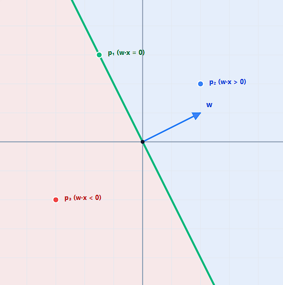
The weight vector $w$ is not the hyperplane itself.

Instead:

$w$ is the normal vector to the hyperplane.

That means:

• $w$ is perpendicular (orthogonal) to the decision boundary
• $w$ determines which side is classified as positive
• the hyperplane is defined relative to $w$

For any two points $x_a,x_b$ lying on the hyperplane:

$w^T{x}_a+b=0$

$w^T{x}_b+b=0$

Subtracting:

$w^T(x_a-x_b)=0$

Thus:

$w$ is perpendicular to every direction lying within the hyperplane. The weight vector defines the orientation and positive direction of the classifier, while the hyperplane itself is the set of points orthogonal to that vector.

The Weight Vector Lies in the Positive Half-Space The hyperplane $w^{T}x=0$ splits space into two regions: Positive half-space: $w^{T}x>0$ Negative half-space: $w^{T}x<0$ The hyperplane equation at $x=w$

		$w^T w = \|w\|^2$
	
		$w^T w > 0$

So the weight vector (w) lies inside the positive half-space defined by the hyperplane. The vector $w$:

• points toward the positive region
• acts as the normal vector to the hyperplane
• defines the direction of increasing score The sign of $w^{T}x$ measures alignment with the weight vector:
• positive dot product → same general direction as $w$
• negative dot product → opposite direction

---

Each perceptron update increases the signed margin of the misclassified point by a strictly positive amount, guaranteeing steady progress toward correct classification (correct side of the decision boundary)

To classify a point correctly, the prediction must agree with the true label. This is captured by requiring:

$y(t)w^{T}x(t)>0$

A point is misclassified when:

$y(t)w^T(t)x(t)<0$

$y(t)w^T(t+1)x(t)>y(t)w^T(t)x(t)$

Proof:

$w(t+1)=w(t)+y(t)x(t)$

$$$y(t)w^T(t+1)x(t) = y(t) \left[ w(t) + y(t)x(t) \right]^T x(t)y(t) \left[ w^T(t) + y(t)x^T(t) \right] x(t)y(t)w^T(t)x(t) + y(t)y(t)x^T(t)x(t)$$

• Since $y(t)$ is either $+1$ or $-1$, its square is always exactly 1.
• The term $x^T(t)x(t)$ is the dot product of a vector with itself, which is equal to its squared length, $\Vert x(t){\Vert }^2$. Assuming the data point is not the origin (a zero vector), this value is strictly positive ($>0$). $y(t)w^T(t+1)x(t)=y(t)w^T(t)x(t)+\Vert x(t){\Vert }^2$ $y(t)w^T(t+1)x(t)>y(t)w^T(t)x(t)$

The score strictly increases after each update.

---

Geometric View of the Perceptron Problem

Each training example imposes a geometric constraint on the weight vector $w$.

For a labeled example $(x_i,y_i)$, correct classification requires:

$y_i{w}^T{x}_i>0$

This can be rewritten as a linear constraint on $w$ (Fix $x_i$, treat w as variable):

$w^T(y_i{x}_i)>0$

The inequality:

$w^T(y_i{x}_i)>0$

defines a half-space in weight space (a half-space of all valid classifiers)** .

We denote it as:

$H_i=\{w:w^T(y_i{x}_i)>0\}$

So each training example restricts $w$ to lie in a convex region.

For a dataset of $N$ examples, we require:

$w\in {\bigcap }_{i=1}^N{H}_i$

This is:

• The set of all perfect classifiers

• $w$ must satisfy all constraints simultaneously

• it must lie in the intersection of all half-spaces

• Each $H_i$ is convex (a half-space is always convex)

• The intersection of convex sets is also convex

The feasible set of solutions is a convex region in weight space

Training becomes:

find a point $w$ inside the intersection of all half-spaces

The perceptron update:

• starts with some $w$
• moves it whenever a constraint is violated
  • if w violates one constraint
  • push w toward satisfying that constraint

The perceptron learning problem is equivalent to finding a point in the intersection of convex half-spaces defined by the training data.

Each training example defines a convex half-space constraint on $w$, and learning reduces to finding a point in the intersection of all such half-spaces.

Perceptron learning is iterative navigation through intersections of convex half-spaces in parameter space, not data space.

---

Why the Perceptron Update Direction is $x$?

Consider the linear objective:

$f(w)=w^{T}x$

where:

• $x$ is fixed
• $w$ is the variable being optimized

We want to determine:

In which direction should we move $w$ to increase $f(w)$ as quickly as possible?

The answer is given by the gradient.

Taking the gradient with respect to $w$:

${\nabla }_w(w^{T}x)=x$

So:

the direction of steepest increase is exactly the vector $x$

$\Delta w\propto x$

If the update is constrained to unit length:

$\Vert \Delta w\Vert =1$

then the optimal direction becomes:

$\Delta w=\frac{x}{\Vert x\Vert }$

which is the normalized version of $x$.

The objective change after a small step $\Delta w$ is:

$(w+\Delta w{)}^{T}x-w^{T}x=\Delta w^{T}x$

So maximizing improvement means maximizing:

$\Delta w^{T}x$

Cauchy–Schwarz Inequality

We use:

$|\Delta w^{T}x|\le \Vert \Delta w\Vert \Vert x\Vert$

If $\Vert \Delta w\Vert =1$, then:

$\Delta w^{T}x\le \Vert x\Vert$

The maximum possible increase is therefore:

$\Vert x\Vert$

Equality in Cauchy–Schwarz occurs only when the vectors are collinear:

$\Delta w=\lambda x$

Under the unit norm constraint:

$\Delta w=\frac{x}{\Vert x\Vert }$

The perceptron update:

$w\leftarrow w+y_t{x}_t$

uses:

• $x_t$ as the optimal correction direction
• $y_t$ to determine whether to move toward or away from the point

Thus:

• positive examples pull $w$ toward themselves
• negative examples push $w$ away

The perceptron update follows the direction that maximally increases the classification score for the current example.

Lagrange Multipliers: Optimal Update Direction

We want to maximize the directional improvement of the objective:

${\max }_{\Delta w}\Delta w^{T}x\text{s.t. }\Delta w^T\Delta w=1$

• Objective: maximize $\Delta w^{T}x$
• Constraint: unit-length update
  $\Vert \Delta w{\Vert }^2=\Delta w^T\Delta w=1$

$L(\Delta w,\lambda )=\Delta w^{T}x-\lambda (\Delta w^T\Delta w-1)$

The Lagrangian says:

“Maximize the objective, BUT punish solutions that break the constraint.”

Differentiate with respect to $\Delta w$:

${\nabla }_{\Delta w}L=x-2\lambda \Delta w=0$

$x=2\lambda \Delta w$

$\Delta w=\frac{1}{2\lambda }x$

Apply unit norm constraint:

$\Vert \Delta w\Vert =1$

Substitute $\Delta w$:

$\Vert \frac{1}{2\lambda }x\Vert =1$

So:

$\frac{1}{2\lambda }\Vert x\Vert =1$

$\frac{\Vert x\Vert }{2\lambda }=1$

$2\lambda =\Vert x\Vert$

$\lambda =\frac{\Vert x\Vert }{2}$

Substitute back into $\Delta w$:

$\Delta w=\frac{1}{2\lambda }x=\frac{1}{\Vert x\Vert }x$

---

If the data is linearly separable:

• PLA is guaranteed to converge
• It will find a valid $w$ in a finite number of steps This result is known as the Perceptron Convergence Theorem.

Perceptron Convergence Theorem :

We are given a dataset $(x_i,y_i)$ where:

• $x_i\in {\mathbb{R}}^d$
• $y_i\in \{-1,+1\}$

We assume linear separability, meaning:

There exists a vector $w^{\ast }$ such that:

$y_i(w^{\ast T}{x}_i)>0\forall i$

Define:

• $R={\max }_i\Vert x_i\Vert$
• $\gamma ={\min }_i{y}_i(w^{\ast T}{x}_i)$ (after normalizing $w^{\ast }$ so $\Vert w^{\ast }\Vert =1$)

So:

• $R$ = maximum data norm (The largest length (magnitude) among all training points)
• $\gamma$ = geometric margin (minimum confidence)

At each mistake on $(x_t,y_t)$:

$w_{t+1}=w_t+y_t{x}_t$

Initialize:

$w_0=0$

We prove two inequalities: (A) Progress toward optimal direction (B) Growth of norm is controlled Combining them gives the mistake bound.

Step 1 - Consider dot product with $w^{\ast }$ (alignment with true solution):

$w_{t+1}^T{w}^{\ast }=(w_t+y_t{x}_t{)}^T{w}^{\ast }$

$w_t^T{w}^{\ast }+y_t{x}_t^T{w}^{\ast }$

So each mistake increases projection by:

$y_t(w^{\ast T}{x}_t)$

By separability:

$y_t(w^{\ast T}{x}_t)\ge \gamma$

So:

$w_{t+1}^T{w}^{\ast }\ge w_t^T{w}^{\ast }+\gamma$

So every mistake pushes $w_t$​ **closer in direction to $w^{\ast }$.

After $M$ mistakes:

$w_M^T{w}^{\ast }\ge M\gamma$

Step 2 - Bound growth of $\Vert w\Vert$

Compute norm growth:

$\Vert w_{t+1}{\Vert }^2=\Vert w_t+y_t{x}_t{\Vert }^2$ = $\Vert w_t{\Vert }^2+2y_t{w}_t^T{x}_t+\Vert x_t{\Vert }^2$

Updates happen only on mistakes, for a mistake:

$y_t{w}_t^T{x}_t\le 0$

So:

$\Vert w_{t+1}{\Vert }^2\le \Vert w_t{\Vert }^2+\Vert x_t{\Vert }^2$

Using $\Vert x_t\Vert \le R$:

$\Vert w_{t+1}{\Vert }^2\le \Vert w_t{\Vert }^2+R^2$

After $M$ mistakes:

$\Vert w_M{\Vert }^2\le M{R}^2$

From Cauchy–Schwarz:

$w_M^T{w}^{\ast }\le \Vert w_M\Vert \Vert w^{\ast }\Vert$

Assume $\Vert w^{\ast }\Vert =1$:

$w_M^T{w}^{\ast }\le \Vert w_M\Vert$

Using bounds:

$M\gamma \le \Vert w_M\Vert \le \sqrt{M}R$

So:

$M\gamma \le \sqrt{M}R$

$\sqrt{M}\gamma \le R$

$M\le \frac{R^2}{{\gamma }^2}$

The number of perceptron mistakes is bounded by: $M\le \frac{R^2}{{\gamma }^2}$

Each update:

• increases alignment with $w^{\ast }$ by at least $\gamma$
• increases weight norm only by at most $R^2$

So:

alignment grows faster than destructive “noise” in magnitude

This forces convergence.

• Larger margin $\gamma$ → faster convergence
• Larger data norm $R$ → slower convergence
• Well-separated data → very few updates

If the data is linearly separable with margin $\gamma$, the perceptron makes at most $\frac{R^2}{{\gamma }^2}$ mistakes before converging.

Even though the hypothesis space is infinite, PLA finds a correct solution using only simple local updates based on misclassified points. So convergence is guaranteed in finite steps.

The perceptron converges because its updates increase alignment with the true separator linearly while controlling norm growth sublinearly, forcing a finite bound on mistakes.

---

Learning from Data vs Design from Specifications

A classic example illustrating the difference between learning from data and design from specifications is coin recognition in vending machines.

The goal is to classify:

• pennies
• nickels
• dimes
• quarters

using:

• coin size
• coin mass

So each coin is represented as a 2D input vector:

$x=(\text{size},\text{mass})$

In the learning approach:

• we collect example coins from each denomination
• each example becomes a labeled training point
• input → size and mass
• output → coin denomination

Coins of the same type form clusters in feature space.

The learning algorithm:

• observes the training data
• searches for a hypothesis $g$
• learns decision boundaries separating the coin classes

A new coin is classified by:

1. measuring size and mass
2. feeding the measurement into the learned classifier

In feature space:

• each denomination forms a cluster
• the classifier partitions the space into regions

The boundaries are inferred directly from data.

In the design approach:

• we use prior knowledge instead of training data
• obtain official specifications from the U.S. Mint
• model:
  • expected coin size
  • expected mass
  • measurement noise
  • wear-and-tear variations
  • relative frequency of each coin

Using this information, we construct a joint probability distribution over:

• size
• mass
• denomination

Once the probability model is known, we analytically derive the optimal classifier.

For a given measurement $(x)$:

choose the denomination with the highest probability:

$\arg {\max }_{y}P(y\mid x)$

This minimizes classification error probability.

In the design approach:

• the problem is fully specified
• we derive the solution mathematically
• Example : Classifying numbers into primes and non-primes, Determining the time it would take a falling object to hit the ground

In the learning approach:

• the target function is unknown
• data is needed to approximate it empirically
• Example : Detecting potential fraud in credit card charges, Determining the age at which a particular medical test should be performed

---

Types of Learning

Learning from data aims to infer an underlying process from observations. Because real-world settings vary widely, different learning paradigms have been developed.

Supervised Learning In supervised learning, each training example includes both:

• input $x$
• correct output $y$

So the dataset has the form:

$(x_i,y_i)$

The learning algorithm uses these labeled examples to approximate the unknown function:

$f:\mathcal{X}\to \mathcal{Y}$

Example: Handwritten Digit Recognition

Each training sample consists of:

• input: image of a digit
• output: label in $\{0,1,2,3,4,5,6,7,8,9\}$

So the dataset is:

$(\text{image},\text{digit})$

The model learns to map images → digit labels.

Active Learning In active learning:

• the algorithm selects inputs $x$
• a supervisor provides the corresponding output $y$ So instead of passively receiving data, the model chooses what to learn from.

The learner can ask strategic questions:

“Which example would be most informative?”

This is similar to a game of 20 questions.

• reduces number of labeled examples needed
• focuses learning on informative regions of the input space

Online Learning

In online learning:

• data arrives sequentially
• the algorithm updates after each example

Instead of seeing a full dataset, the learner processes a stream:

$(x_1,y_1),(x_2,y_2),\dots$

The model must:

• learn continuously
• update in real time

Use Cases

• streaming recommendation systems
• real-time user feedback (e.g., clicks, ratings)
• systems with memory or compute constraints
• no full dataset is required

---