Optimization Theory

Given a differentiable objective function:

$f:{\mathbb{R}}^n\to \mathbb{R}$

The target is to locate an optimal vector $x$ within a designated feasible set $M\subseteq {\mathbb{R}}^n$:

${\min }_{x\in {\mathbb{R}}^n}f(x)\text{subject to }x\in M$

The boundaries of the feasible set $M$ are algebraically constructed via finite sets of equality and inequality constraints: $M:=\left\{x\in {\mathbb{R}}^n|[cit{e}_{s}tart]\begin{array}{rlrl}{h}_i(x)& =0& & \text{for }i\in I\\ g_j(x)& \ge 0& & \text{for }j\in J\end{array}\right\}$

• $I$ and $J$ represent discrete, finite index sets.
• The constraint mappings $h_i,g_j:{\mathbb{R}}^n\to \mathbb{R}$ are assumed to be sufficiently smooth and continuously differentiable.

An optimization problem is classified as unconstrained if the feasible set encompasses the entire unrestricted vector space:

$\text{If }M={\mathbb{R}}^n⟹{\min }_{x\in {\mathbb{R}}^n}f(x)$

Under unconstrained conditions, solutions are analyzed using localized neighborhood behaviors rather than boundary intersections.

Unconstrained Local Optima (LOCAL MINIMA)

• A point $x\in {\mathbb{R}}^n$ represents a strict local minimum of a function if it yields the lowest scalar evaluation within an isolated domain.
• An element $x\in {\mathbb{R}}^n$ is a local minimum of $f:{\mathbb{R}}^n\to \mathbb{R}$ if and only if there exists a localized open neighborhood, parameterized as an $ϵ$-ball ($B_{ϵ}$): $B_{ϵ}(x):=\{y\in {\mathbb{R}}^n\mid \Vert x-y\Vert [cit{e}_{s}tart]<ϵ\}\text{for }ϵ>0$ Such that the following optimality condition holds strictly for all surrounding coordinates: $\forall y\in B_{ϵ}(x),f(x)\le f(y)$

To mathematically verify that an unconstrained point is a local minimum, look at how the function behaves if you take a tiny step in any direction away from that point ($B_{ϵ}$). This neighborhood analysis relies on two conditions :

1. The First Derivative Condition (Gradient): The slope at that exact coordinate must flatten out completely: $\nabla f(x)=0$
   • The gradient vector ($\nabla f(x)$ or $Df(x)$) collects all the first partial derivatives, telling the steepness and direction of the slope.
   • x is a critical point and it may correspond to a local maximum, a local minimum, or a saddle/inflection point.

When optimizing in multiple dimensions (like a neural network with many weights), looking at a single slope value is not enough to understand the surrounding terrain.

2. The Second Derivative Condition (Hessian Matrix): To confirm it is a local minimum, you analyze the curvature in a neighborhood of the point.
   • The Hessian Matrix ($D^{2}f(x)$) has all the second partial derivatives. This matrix must be positive definite. This means that no matter which direction you look inside your localized neighborhood ball, the ground curves upward away from x.
   • In an $n$-dimensional space, the Hessian is a square $n\times n$ symmetric matrix :

$D^{2}f(x)=\left(\begin{array}{cccc}\frac{{\partial }^{2}f}{\partial x_1^2}& \frac{{\partial }^{2}f}{\partial x_1\partial x_2}& \cdots & \frac{{\partial }^{2}f}{\partial x_1\partial x_n}\\ \frac{{\partial }^{2}f}{\partial x_2\partial x_1}& \frac{{\partial }^{2}f}{\partial x_2^2}& \cdots & \frac{{\partial }^{2}f}{\partial x_2\partial x_n}\\ ⋮& ⋮& \ddots & ⋮\\ \frac{{\partial }^{2}f}{\partial x_n\partial x_1}& \frac{{\partial }^{2}f}{\partial x_n\partial x_2}& \cdots & \frac{{\partial }^{2}f}{\partial x_n^2}\end{array}\right)$ - The Diagonal Terms ($\frac{{\partial }^{2}f}{\partial x_i^2}$): Measure how the slope is curving if you walk strictly parallel to one of the main coordinate axes. - The Cross Terms ($\frac{{\partial }^{2}f}{\partial x_i\partial x_j}$): Measure how the slope changes in one direction as you move in a different direction (the twist or rotation of the terrain).

The Sufficient Second Order Conditions for a local minimum:

Let $x^{\ast }\in {\mathbb{R}}^n$ be twice differentiable with $Df(x^{\ast })=0$ and let $D^{2}f(x^{\ast })$ be positive definite. Then $x^{\ast }$ is a local minimum of $f$.

For a symmetric matrix $A$ (Hessian $D^{2}f(x^{\ast })$) to be positive definite, it must satisfy for every non-zero vector $x\in {\mathbb{R}}^n$: $x^{T}Ax>0(\text{or }{v}^T[D^{2}f(x^{\ast })]v>0)$

• $v$: A vector representing a step in any random direction you choose to walk inside your localized neighborhood ball.
• $[D^{2}f(x^{\ast })]v$: Multiplies your step direction by the curvature matrix, figuring out how the slopes alter along that specific path.
• $x^{\ast }\in {\mathbb{R}}^n$ is a specific, fixed coordinate in your parameter space where you are currently standing. It is the exact point you are testing to see if it is a local minimum.
• The $x$ in $x^{T}Ax>0$ is a variable vector representing a step in any arbitrary direction away from your anchor point $x^{\ast }$.

The resulting output ($v^T[D^{2}f(x^{\ast })]v$) is a single scalar number that represents the directional second derivative.

• If this value is strictly greater than zero ($>0$) for every single possible vector $v$, it means that no matter which compass heading you choose to step toward, the slope immediately starts tilting upward Caveat : If you find a local minimum, its Hessian matrix does not have to be strictly positive definite.
• If $D^{2}f(x^{\ast })>0⟹$ It is guaranteed to be a local minimum (Sufficient).
• If it is a local minimum $⟹$ $D^{2}f(x^{\ast })$ can be $>0$ OR it can be exactly $=0$ (like $f(x)=x^4$).

Because derivatives only look at an infinitely small neighborhood ($B_{ϵ}$), passing these tests only proves you are at the bottom of a valley. It does not tell you if there is a much deeper valley somewhere else on the map. To guarantee a global optimum we must look at the convexity condition.

Constrained Optimization The optimal points lie on the boundaries of the feasible set, not at a local stationary point where the derivative vanishes.

In constrained optimization, the optimal point does not occur at an interior stationary point where $\nabla f=0$. Instead, it lies on the constraint $h(x)=0$.

At the optimal point $(x^{\ast },y^{\ast })$, the constraint curve and the level curve of the objective function $f$ are tangent to each other. Because they are tangent, their gradient vectors $\nabla f$ and $\nabla h$ must be parallel at that point (parallel meaning they lie along the same line, but may point in the same or opposite directions).

This parallelism condition is written as: $\nabla f(x^{\ast })=\lambda ,\nabla h(x^{\ast })$ where $\lambda \in \mathbb{R}$ is a scalar constant called the Lagrange multiplier. It can be positive or negative depending on whether the gradients point in the same or opposite directions.

The Lagrangian Function

To find the optimal point systematically, we construct the Lagrangian: $\mathcal{L}(x,\lambda )=f(x)-\lambda h(x)$ This reformulates the original constrained problem into an unconstrained one — we simply look for points where $\nabla \mathcal{L}=0$. This gives a system of equations: $\frac{\partial \mathcal{L}}{\partial x}=0\Rightarrow \nabla f(x)=\lambda \nabla h(x)$ $\frac{\partial \mathcal{L}}{\partial \lambda }=0\Rightarrow h(x)=0$

Lagrange with One Equality Constraint Theorem: Let $f,h:{\mathbb{R}}^n\to \mathbb{R}$ be continuously differentiable functions. Let $\bar{x}$ be a local optimum of $f$ under the constraint $h(x)=0$. If $Dh(\bar{x})\ne 0$, then there exists a Lagrange parameter $\lambda \in \mathbb{R}$ such that: $Df(\bar{x})=\lambda \cdot Dh(\bar{x})$

If $Dh(\bar{x})$ became zero, the boundary line would disappear into a flat plain, making it impossible to align vectors. This requirement is called a Constraint Qualification.

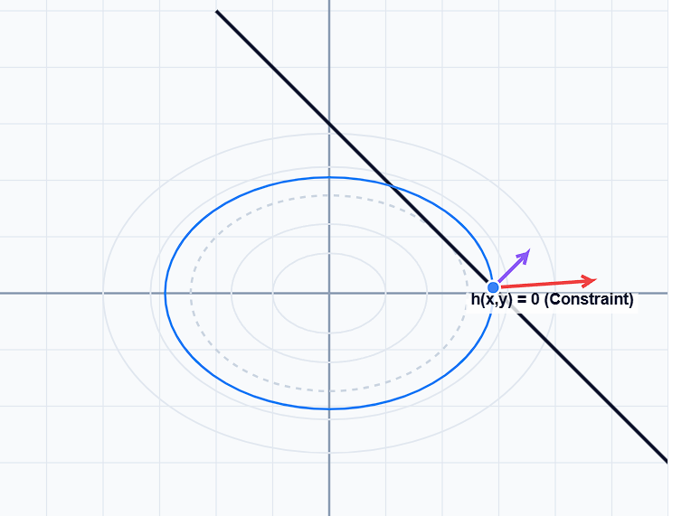
The geometric intuition behind finding an optimum for functions in two variables ($f,h:{\mathbb{R}}^2\to \mathbb{R}$). Contour lines (level curves) for the objective function $f$ at various values (e.g., $f=-5$, $f=1.5$, f=2$,$f=3$).Overlaidonthisisathickercurverepresentingtheconstraintsetwhere$h(x, y) = 0$.

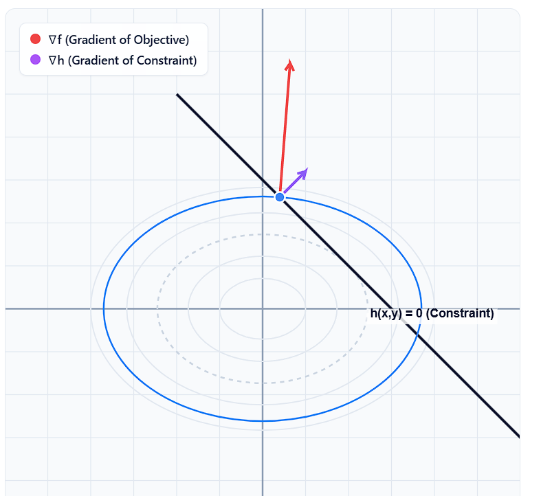
• Transverse Intersections (Not Optimal): The notes point to a location where the constraint curve $h=0$ simply crosses through the level curves of $f$ (like $f=3$ and $f=2$). At these intersections, the text explains: “This will not be a local optimum of $f$ under constraints $h(x,y)=0$, bcz we can move along $\{(x,y)\mid h(x,y)=0\}$ and decrease/increase $f$.” If the curves cross transversally, you can simply slide along the $h=0$ path to reach a lower or higher contour line of $f$.

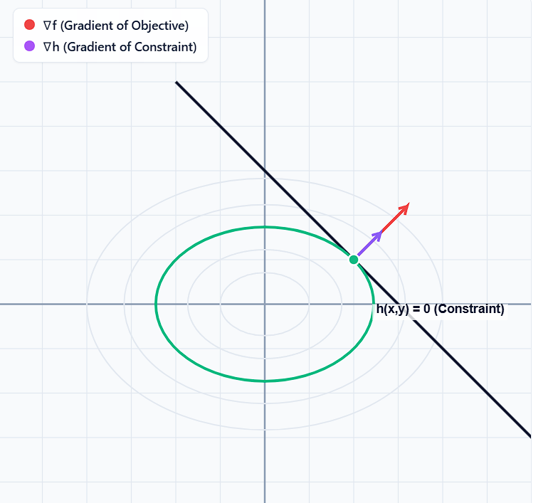
• Tangential Intersections (The Optimum): The diagram highlights a specific point $(x^{\ast },y^{\ast })$ where the level curve $f=1.5$ merely touches the constraint curve $h=0$ without crossing it. At this point, the gradient vectors $\nabla h(x^{\ast },y^{\ast })$ and $\nabla f(x^{\ast },y^{\ast })$ are drawn pointing in parallel/anti-parallel directions.

---

To solve a constrained problem via Lagrange multipliers, we match our equations to our unknowns:

• Vector Alignment: $Df(\bar{x})=\lambda Dh(\bar{x})$ yields $n$ equations.
• Constraint Boundary: $h(\bar{x})=0$ yields $1$ additional equation.
• Total: $n+1$ equations for $n+1$ unknowns (the vector coordinates $\bar{x}$ and the scalar $\lambda$).

Steepest Descent When analytical solutions are impossible, we use a step-by-step algorithm to approximate local optima:

1. Initialize: Choose an arbitrary starting point $x_0\in {\mathbb{R}}^n$.
2. Direction Selection: At your current position $x_k$, calculate a downward search direction vector $g_k$ such that the function decreases: $\text{Direction: }{g}_k\in {\mathbb{R}}^n$
3. Position Update (The Step): Compute your next location using the update rule: $x_{k+1}=x_k+t_k\cdot g_k$ Where $t_k>0$ is the step length (Learning Rate).
4. Termination: Halting criteria triggers when the gradient norm approaches zero ($\Vert \nabla f(x_k)\Vert \approx 0$).

The absolute best direction is the negative gradient ($-\nabla f(x)$).

• Given a smooth, differentiable function $f:{\mathbb{R}}^n\to \mathbb{R}$.
• At a position $x\in {\mathbb{R}}^n$ where the ground is not flat: $Df(x)\ne 0$.
• Pick an arbitrary direction vector $g \in \mathbb{R}^n$$$ \sqrt{g^T g} = |g| = 1$$
• The directional derivative of $f$ in $x$ into direction $g$ is $Df(x)\cdot g$
• To find the steepest descent, we want to find the direction $g^{\ast }$ that makes this directional derivative as small (as deeply negative) as possible
• The first-order Taylor expansion approximation: $f(x+g)=f(x)+DF(x)\cdot g+O(\Vert g{\Vert }^2)$ We have a constrained optimization problem where the step direction $g$ is the variable we want to solve for. ${\min }_{g}DF(x)\cdot g\text{subject to}{g}^{T}g-1=0$ The Objective Function: $DF(x)\cdot g$ (Goal is to minimize this function) The Constraint ($h(g)=0$): $g^{T}g-1=0⟹\Vert g{\Vert }^2=1$

$\text{Gradient of Objective w.r.t. }g⟹DF(x)$

$\text{Gradient of Constraint }h(g)\text{ w.r.t. }g⟹{\nabla }_g(g^{T}g-1)=2g$

Plugging these into the Lagrange formula ($Df=\lambda Dh$):

$DF(x)=\lambda \cdot (2g^{\ast })$ $DF(x)=\lambda \cdot g^{\ast }$

This equation tells us that the optimal step direction $g^{\ast }$ must point along the exact same line as our gradient vector $DF(x)$. Because our constraint forces the length of $g^{\ast }$ to be exactly $1$ ($\Vert g^{\ast }\Vert =1$)

$\Vert DF(x)\Vert =|\lambda |\cdot \underset{1}{\underbrace{\Vert g^{\ast }\Vert }}⟹|\lambda |=\Vert DF(x)\Vert$ $\lambda =\pm \Vert DF(x)\Vert$

From our original equation $DF(x)=\pm \Vert DF(x)\Vert \cdot g^{\ast }$ We get

1. The Uphill Direction : $g^{\ast }=\frac{DF(x)}{\Vert DF(x)\Vert }$
2. The Downhill Direction : $g^{\ast }=-\frac{DF(x)}{\Vert DF(x)\Vert }$

To find out which one minimizes our objective function, we plug both options back into our directional derivative $DF(x)\cdot g$:

• If we plug in Option 1, we get a positive number (steepest ascent).

• If we plug in Option 2, we get a negative number: $-\frac{DF(x)\cdot DF(x)}{\Vert DF(x)\Vert }=-\Vert DF(x)\Vert$ (steepest descent).

• $g^{\ast }=-\frac{Df(x)}{\Vert Df(x)\Vert }$

• The raw gradient vector $Df(x)$ naturally points straight uphill (steepest ascent). A negative sign flips the arrow completely around so it points straight downhill (steepest descent).

---

Steepest descent is an important iteration procedure which is for example used in the Backpropagation algorithm.

As you cannot analytically calculate the perfect weights for a neural network all at once. Instead, you map out a massive error landscape called a Loss Function, $L(w)$.

1. The Forward Pass: The network makes a prediction, and you calculate the total error ($f(x)$ in your notes represents this loss value).
2. The Backward Pass (Backpropagation): The algorithm uses the chain rule to compute the exact partial derivatives of that error with respect to every single weight in the model. This compiles the giant gradient vector, $DF(w)$.
3. The Step (Steepest Descent): We then flips that gradient vector around to find the direction of steepest descent ($g^{\ast }=-DF(w)$) and shifts the weights of the network a tiny fraction in that direction to minimize the error.

---

Optimization Under Inequality Constraints : Karush-Kuhn-Tucker (KKT) Conditions

When optimizing an objective function $f(x)$ subject to inequality constraints $g_j(x)\ge 0$, the feasible region is defined by a set of inequalities. To characterize the local optima within this region, the classical Lagrange multiplier approach is generalized into the Karush-Kuhn-Tucker (KKT) conditions.

Simple Analogy : When a constraint is an equality ($h(x)=0$), you are forced to walk exactly on top of a thin fence. When a constraint is an inequality ($g_j(x)\ge 0$), you are dealing with an entire allowable region (a yard). You can walk anywhere inside the yard ($g_j(x)>0$), or you can walk right up against the perimeter fence ($g_j(x)=0$).

At any candidate local minimum $\bar{x}$, the constraint set $J$ is partitioned based on the evaluation of $g_j(\bar{x})$:

• Active Constraints ($J_0$): Defined as $J_0(\bar{x})=\{j\in J\mid g_j(\bar{x})=0\}$. The candidate point lies exactly on the boundary of these constraints.

• Inactive Constraints: Constraints where $g_j(\bar{x})>0$. The candidate point lies strictly in the interior of the feasible region with respect to these boundaries.

• Regularity Condition (LICQ): We assume the Linear Independence Constraint Qualification holds; specifically, the gradients of all active constraints, $\{D{g}_j(\bar{x})\mid j\in J_0(\bar{x})\}$, are linearly independent.

  • The Linear Independence Constraint Qualification (LICQ) is a regularity condition in nonlinear optimization. At a feasible point x∗ for a problem with equality constraints h(x)=0 and inequality constraints $g_j(x)\ge 0$, LICQ holds if the set of gradients of all equality constraints and of all active inequality constraints is linearly independent.
  • When LICQ holds at a local minimizer, KKT multipliers exist and are unique.

The Stationarity Condition : At a local minimum $\bar{x}$, the gradient of the objective function must be equal to a linear combination of the gradients of the active constraints:

$Df(\bar{x})={\sum }_{j\in J_0(\bar{x})}{\mu }_j\cdot D{g}_j(\bar{x})$

• $Df(\bar{x})$: The gradient vector of your objective function. It points in the direction of steepest ascent.
• $D{g}_j(\bar{x})$: The gradient vectors of your active constraints (the boundaries you are physically touching).
• ${\mu }_j$: The scaling weights (Lagrange multipliers) for those active constraints
• Non-Negativity of Multipliers: Unlike equality constraints, the KKT multipliers for inequalities must be non-negative (${\mu }_j\ge 0$). This ensures that the gradient of the objective function is opposed exclusively by vectors pointing inward toward the feasible region, preventing further descent.

To unify the stationarity condition across the entire constraint set $J$ (without explicitly partitioning $J_0$), we introduce the Complementary Slackness condition:

${\mu }_j\cdot g_j(\bar{x})=0,\forall j\in J$

• If a constraint is inactive ($g_j(\bar{x})>0$, If there is Slack), its corresponding Lagrange multiplier must be strictly zero (${\mu }_j=0$), eliminating its gradient from the stationarity equation.
• If a constraint is active ($g_j(\bar{x})=0$), its corresponding Lagrange multiplier may be positive (${\mu }_j\ge 0$).

Identifying exactly which constraints belong to the active set $J_0$ beforehand is computationally difficult for a computer.

By enforcing Complementary Slackness (${\mu }_j{g}_j=0$), we don’t have to partition the constraints into “active” and “inactive” sets. We can rewrite the earlier stationarity condition to sum over every single constraint in the entire system (the set $J$):

$Df(\bar{x})={\sum }_{j\in J}{\mu }_j\cdot D{g}_j(\bar{x})$

An active inequality constraint is simply a temporary equality constraint that only works in one direction.

If your algorithm’s objective function gradient is trying to drag you into the wall, the wall pushes back (μ>0). But if your algorithm decides to turn around and walk back into the grass, the wall instantly stops affecting you, the constraint becomes inactive, and its multiplier drops to zero (μ=0).

---

Convexity If an optimization problem is convex, it is mathematically guaranteed that any local minimum is also the absolute global minimum.

To prove an optimization problem is convex, you must prove two things:

1. The feasible region is a Convex Set.
2. The objective function is a Convex Function.

Theorem: Let $M\in {\mathbb{R}}^n$ be a convex set, and $f:M\to \mathbb{R}$ be a convex function. Then, every local minimum of $f$ on $M$ is strictly also a global minimum.

Formal Proof (By Contradiction)

Suppose $x\in M$ is a local minimum of $f$. By definition, there exists a local neighborhood (a ball $U$) around $x$ such that for all points inside that neighborhood, $x$ is the lowest point: $\forall y\in U\cap M,f(y)\ge f(x)$ Suppose for the sake of contradiction that $x$ is not the global minimum. This means there must exist some other point $z\in M$ that is strictly lower: $f(z)<f(x)$ Because $M$ is a convex set, the line connecting $x$ and $z$ lies entirely within $M$. Let us pick a point $y$ on this line that is close enough to $x$ that it falls inside our local neighborhood $U$:

$y=\lambda x+(1-\lambda )z\in U\text{for some }\lambda \in (0,1)\text{ near }1$

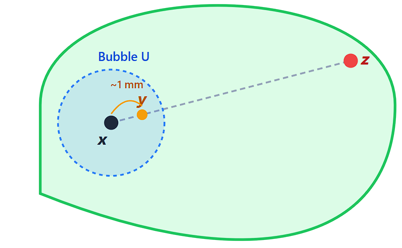
Because $f$ is a convex function, we apply Jensen’s inequality to our point $y$:

$f(y)=f(\lambda x+(1-\lambda )z)\le \lambda f(x)+(1-\lambda )f(z)$

Because our assumption in Step 2 stated that $f(z)<f(x)$, we can replace $f(z)$ with $f(x)$ to make the right side of the equation strictly larger:

$f(y)<\lambda f(x)+(1-\lambda )f(x)$ $f(y)<(\lambda +1-\lambda )f(x)$ $f(y)<f(x)$ We have just proven that $f(y)<f(x)$ for a point $y$ inside the neighborhood $U$. However, this fundamentally contradicts our starting definition that $x$ is the local minimum of $U$. Because this contradiction exists, our assumption that a lower point $z$ exists must be false. Thus, the local minimum $x$ must be the global minimum.

The First-Order Characterization: A differentiable function is convex if and only if
its graph lies strictly on or above all of its tangent hyperplanes.

f(x) ≥ f(x₀) + f'(x₀)(x - x₀)

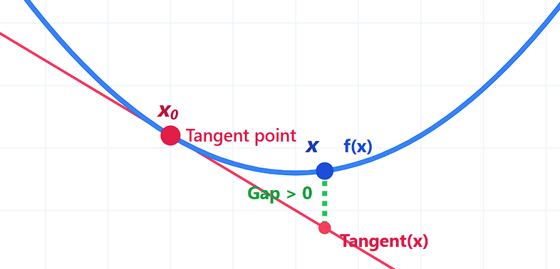
For non-convex functions, $Df(x)=0$ is merely a necessary condition for a local minimum. For convex functions, it is both necessary and sufficient for a global minimum.

This proves that making a local linear approximation of a convex function always safely underestimates the actual cost.

Linear constraints ($Ax\le b$) form convex feasible regions (polyhedrons), and linear objective functions ($\min c^{T}x$) are convex, the entire Linear Programming problem is convex.

The Fundamental Theorem of Linear Programming.

If a linear programming problem has an optimal solution and its feasible region is non-empty and bounded (or more generally, if an optimum exists), then: At least one optimal solution occurs at a vertex (extreme point) of the feasible polytope.

Because both your goal (the tilted floor) and your boundaries (the straight fences) are strictly linear, the absolute lowest or highest point is mathematically guaranteed to be at an extreme point (a corner)

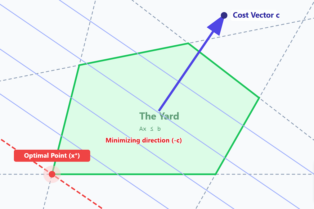
• The purple arrow represents the direction that “increases” the cost. Since we want to minimize cost, we want to go in the exact opposite direction.
• The dashed red line represents all the points in the universe that share the exact same cost right now. It sits perfectly perpendicular to the cost vector.
• The linear function we are trying to minimize ($c^{T}x$) is perfectly flat and straight, like a tilted floor. Because it doesn’t have any curves, bowls, or dips, a ball rolling on this floor will never stop in the middle of the yard. It will always keep rolling downhill until it hits a wall
• The fences ($Ax\le b$) are also perfectly straight lines. There are no curved walls to gently cradle the ball.

---

The Quadratic Function ($x^{T}Dx$) : The function is convex if and only if the matrix $D$ is Positive Semi-Definite (PSD). The shape of the landscape is dictated entirely by the matrix $D$.

Trying to minimize a general quadratic function $f(x)=x^{T}Dx$ over a positive boundary ($x\ge 0$) is NP-hard if $D$ is not restricted to being Positive Semi-Definite.

---

The Least Mean Square (LMS) Algorithm :

The algorithm relies on the Adaptive Linear Element (ADALINE) architecture:

• Input Layer: $n$ neurons receiving input vector $X\in {\mathbb{R}}^n$.
• Output Layer: $1$ single continuous neuron.
• Weights: Vector $w\in {\mathbb{R}}^n$. No bias term is used.
• Activation Function: Linear identity function $\phi (t)=t$.
• Forward Pass (Prediction): $y=w^{T}X$

The LMS algorithm processes streaming data in discrete timesteps ($k\ge 0$):

• Inputs: Randomly sampled vectors $X^{(k)}\in {\mathbb{R}}^n$.
• Targets: The desired true scalar value $d^{(k)}\in \mathbb{R}$.
• The underlying probability distribution governing how $X$ and $d$ are generated is strictly unknown.

The Objective Function : At each timestep $k$, the current weight vector $w^{(k)}$ is used to approximate the target

• The Instantaneous Error ($\epsilon$):$\epsilon (X^{(k)})=d^{(k)}-(w^{(k)}{)}^T{X}^{(k)}$
• $X^{(k)}$ and $d^{(k)}$ are drawn from an unknown probability distribution, the squared error ${\epsilon }^2(X^{(k)})$ is a random variable.
• The Optimization Goal: The algorithm seeks to adjust the weights to minimize the Expected Squared Error: ${\min }_w\mathbb{E}\left[{\epsilon }^2(X^{(k)})\right]$ $\mathbb{E}\left[{\epsilon }^2(x^{(k)})\right]=J(w)$

LMS is a quadratic optimization problem :

${\epsilon }^2={\left(d-w^{T}X\right)}^2$ ${\epsilon }^2=d^2-2d(X^{T}w)+(w^{T}X)(X^{T}w)$ ${\epsilon }^2=w^T\left(X{X}^T\right)w-2\left(d{X}^T\right)w+d^2$ The weights $w$ are constants that we control at any given step, the expectation only acts on the random data variables ($X$ and $d$):

$\mathbb{E}[{\epsilon }^2]=w^T\underset{\mathbf{R}}{\underbrace{\mathbb{E}\left[X{X}^T\right]}}w-2\underset{\mathbf{p}}{\underbrace{\mathbb{E}\left[d{X}^T\right]}}w+\underset{c}{\underbrace{\mathbb{E}[d^2]}}$ We have a multi-dimensional quadratic polynomial equation:

$\mathbb{E}[{\epsilon }^2]=w^T\mathbf{R}w-2{\mathbf{p}}^{T}w+c$

• The Quadratic Matrix ($\mathbf{R}$): $\mathbf{R}=\mathbb{E}[X{X}^T]$ (Correlation Matrix of the input signals, $D$ in $x^{T}Dx$).
• The Linear Vector ($\mathbf{p}$): $\mathbf{p}=\mathbb{E}[dX]$ (Cross-Correlation Vector) between the input signals and the true target. It determines where the center of the bowl shifts in space.
• The Constant ($c$): $\mathbb{E}[d^2]$ is simply the total power of the target signal.

A quadratic problem is only efficiently solvable (convex) if the matrix is Positive Semi-Definite (PSD).

For any arbitrary vector $h$:

$h^T\mathbf{R}h=h^T\mathbb{E}[X{X}^T]h=\mathbb{E}[(h^{T}X)(X^{T}h)]=\mathbb{E}[(h^{T}X{)}^2]\ge 0$

The matrix $\mathbf{R}$ is guaranteed to be Positive Semi-Definite. LMS forms a perfect, error-free convex bowl with a single global minimum. The steepest descent algorithm will never get trapped.

Stationarity Assumption : For the expectation operator $\mathbb{E}[\cdot ]$ to be valid over time, we must assume the data stream is Wide-Sense Stationary. The statistical properties (mean and variance) of the random input vectors $x^{(k)}$ and the targets $d^{(k)}$ do not shift or change as time $k$ progresses.

$J(w)=\mathbb{E}\left[(d^{(k)}{)}^2\right]+w^T\mathbb{E}\left[x^{(k)}(x^{(k)}{)}^T\right]w-2w^T\mathbb{E}\left[d^{(k)}{x}^{(k)}\right]$ $J(w)=\mathbb{E}\left[(d^{(k)}{)}^2\right]+w^T{R}_{x}w-2w^T{P}_x$ $D_{w}J(w^{\ast })=2R_x{w}^{\ast }-2P_x=0$ $R_x{w}^{\ast }=P_x$ Assuming the correlation matrix $R_x$ is invertible (meaning the inputs are not perfectly redundant)

Wiener-Hopf Solution: $w^{\ast }=R_x^{-1}{P}_x$ Computing the inverse of a massive matrix ($R_x^{-1}$) takes an incredible amount of computer memory and processing time. To bypass the matrix inversion bottleneck, we apply the Steepest Descent algorithm. Instead of calculating the inverse, the algorithm iteratively updates the weights by stepping in the opposite direction of the gradient.

The Iterative Solution (Gradient Descent) :

• The Gradient: $D_{w}J(w)=2R_{x}w-2P_x$
• The Update Rule: $w^{(i+1)}=w^{(i)}-\eta \cdot \left(2R_x{w}^{(i)}-2P_x\right)$ $\eta >0$ is the learning parameter

Because the objective function is strictly convex (as $R_x$ is Positive Semi-Definite), this gradient descent formulation is mathematically guaranteed to converge to the true Wiener-Hopf solution ($w^{\ast }$), provided that the learning parameter $\eta$ is chosen correctly (neither too large nor too small).

Problem : As we don’t know the probability distribution, we literally cannot calculate $R_x$ or $P_x$ (in either the Wiener-Hopf inverse matrix or the Gradient Descent loop).

1. Estimation Approach (Batch Gradient Descent) : Collect a massive batch of data points (size $S$). You take all those samples and average them together to create “fake” versions of $R_x$ and $P_x$. While the Law of Large Numbers guarantees these converge to the true $R_x$ and $P_x$ as $S\to \infty$, It requires storing millions of data points in memory and waiting incredibly long times before you can take a single step downhill.

   • Estimated Autocorrelation: $R^{(S)}=\frac{1}{S}{\sum }_{i=1}^S{x}^{(i)}(x^{(i)}{)}^T$

   • Estimated Cross-Correlation: $P^{(S)}=\frac{1}{S}{\sum }_{i=1}^S{d}^{(i)}{x}^{(i)}$

2. The Widrow-Hoff Approach (Stochastic Gradient Descent) : Use the one single data point we have right now ($x^{(k)}$ and $d^{(k)}$). We drop the Expectation operator $\mathbb{E}[\cdot ]$ entirely and calculate the instantaneous squared error for the single incoming data point: ${\epsilon }^2(x^{(k)})={\left(d^{(k)}-w^{(k)}\cdot x^{(k)}\right)}^2$

   • The Gradient: ${\nabla }_w({\epsilon }^2)=-2\cdot \epsilon (x^{(k)})\cdot x^{(k)}$

       			$\varepsilon\!\left(x^{(k)}\right) = d^{(k)} - w^T x^{(k)}$
       			
       			$\varepsilon^2\!\left(x^{(k)}\right) = \left(d^{(k)} - w^T x^{(k)}\right)^2$
       			
       			$\nabla_w \varepsilon^2\!\left(x^{(k)}\right) = 2\left(d^{(k)} - w^T x^{(k)}\right)\nabla_w\!\left(d^{(k)} - w^T x^{(k)}\right)$
       			
       			$\nabla_w\!\left(d^{(k)} - w^T x^{(k)}\right) = -x^{(k)}$
       			
       			$\nabla_w \varepsilon^2\!\left(x^{(k)}\right) = 2\left(d^{(k)} - w^T x^{(k)}\right)\left(-x^{(k)}\right)$
       			
       			$\boxed{\nabla_w \varepsilon^2\!\left(x^{(k)}\right) = -2\,\varepsilon\!\left(x^{(k)}\right)x^{(k)}}$
     

• The Update Equation: Substituting this into the standard steepest descent formula ($w-\eta \nabla J$) : w^{(k+1)} = w^{(k)} - \eta \cdot [ \text{Gradient} ]$$$$w^{(k+1)} = w^{(k)} + 2 \cdot \eta \cdot \varepsilon(x^{(k)}) \cdot x^{(k)} The algorithm operates strictly on-line. It integrates new data points $x^{(k)}$ one at a time and adapts the weights instantly without needing prior knowledge of the environment’s probability distribution. (“Goldfish” Algorithm (Read, Update, Delete))

Brownian Motion: The trajectory of the weight vector $w^{(k)}$ forms a stochastic process. The sequence of updates resembles Brownian motion (a random walk) as it navigates the error surface. Convergence: Due to this stochastic noise, the weights do not perfectly freeze at the absolute minimum $w^{\ast }$. Instead, the algorithm converges in the mean, meaning the expected value of the weights approaches the optimal Wiener-Hopf solution: $\mathbb{E}[w^{(k)}]\to w^{\ast }$.

For the LMS algorithm to remain stable and converge (in the mean) to the optimal solution, the fixed learning parameter $\eta$ must satisfy a strict boundary condition:

$0<\eta <\frac{1}{{\lambda }_{max}}$

• ${\lambda }_{max}$ is the largest eigenvalue of the true autocorrelation matrix $R_x$ (representing the steepest curve of the quadratic bowl).

Because the underlying distribution is unknown, $R_x$ (and thus ${\lambda }_{max}$) is generally unknown. Therefore, $\eta$ must be tuned empirically in practice to ensure it doesn’t exceed this hidden boundary and cause the algorithm to diverge. While the theoretical derivation of the objective function $J(w)$ assumed a stationary environment, the iterative, memory-less nature of the LMS update rule allows it to effectively track optimal weights in non-stationary environments (where the underlying data distribution slowly shifts over time).

---

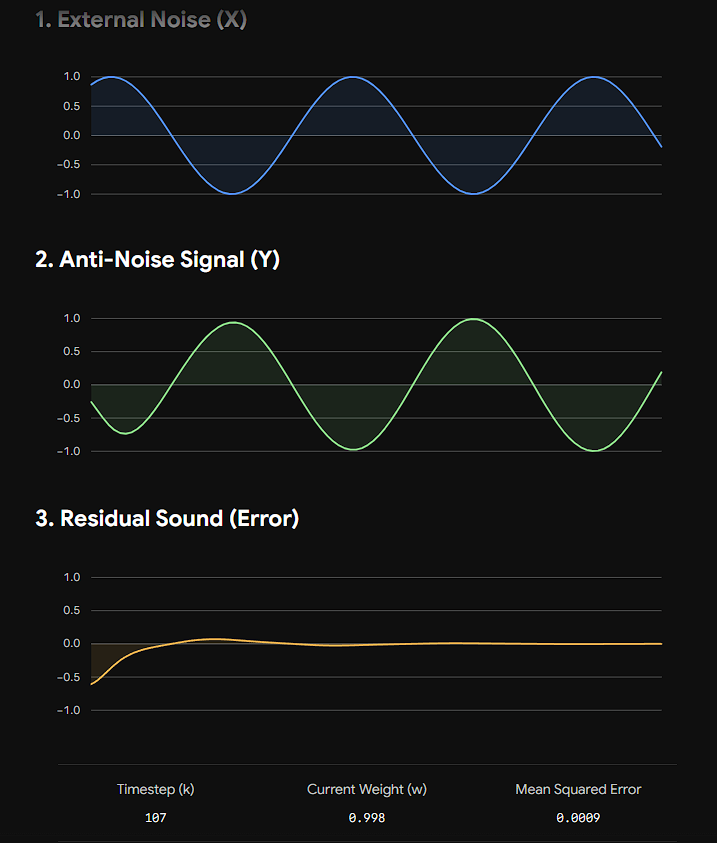
Example Least Mean Square (LMS) algorithm is most famous: Signal Processing and Active Noise Cancellation A pair of noise-canceling headphones has a version of the LMS algorithm running.

The Streaming Input ($X^{(k)}$) : At timestep $k=1$).

The ADALINE chip inside the headphones takes that raw noise $X^{(k)}$ and multiplies it by its current weight ($w$). This calculation generates a new sound wave (the “anti-noise”) and immediately plays it through the speaker into your ear. The anti-noise is the prediction: $w^T{X}^{(k)}$.

The “true target” for noise cancellation is $d^{(k)}=0$ (Silence)

Error: $\epsilon =d^{(k)}-y_{pred}$ (Target Silence - Actual Leftover Hum).

The LMS algorithm takes that tiny error, tweaks its weights $w$ just a fraction of an amount, and gets ready for Millisecond 2 ($k=2$).

The headphones do not have the complex aerodynamic physics equations of a Boeing 737 jet engine programmed into them. The probability distribution of the engine’s roar is completely unknown. The headphones also don’t know the exact physical shape of your unique ear canal. By processing the stream of data one discrete timestep at a time. The LMS algorithm adapts and within a few hundred milliseconds, it figures out the pattern, the error drops to zero, and the airplane goes silent.