Eigenvectors and Eigenvalues
A matrix represents a linear transformation. An eigenvector of a square matrix is a non-zero vector that, when the matrix is multiplied by , the direction of is unchanged.
The result is simply the original vector scaled by some number .
This number is the eigenvalue corresponding to the eigenvector .
Eigenvalues are defined only for square matrices
Mathematical Formulation
The defining equation is:
where:
- is an square matrix
- is the eigenvector
- is the eigenvalue (can be zero, negative, or complex)
Geometric Interpretation
When a matrix transforms most vectors, it both rotates and scales them. But eigenvectors are special:
- They only get scaled (stretched or shrunk)
- Their direction remains the same (or flips if )
Simple 2×2 Example
Consider:
Eigenvector 1:
Check:
So ✓
Eigenvector 2:
Check:
So ✓
Finding Eigenvalues and Eigenvectors
Step 1: Find Eigenvalues
Rearrange to:
For non-zero to exist, the matrix must be singular:
This gives the characteristic equation.
Step 2: Find Eigenvectors
For each eigenvalue , solve:
The solutions (excluding ) are the eigenvectors.
Simplifying Computations
- Powers of matrices:
- Matrix exponentials:
Proof (by induction on k)
- Base cases:
- : .
- : (by definition).
- Inductive step: Assume for some . Then Hence, by induction, for all .
If is invertible, the identity extends to all integers :
since and the same induction applies.
Conceptual view
An eigenvector specifies an invariant one-dimensional subspace (an “axis”) of the transformation . Acting by on that axis is simply scaling by . Reapplying times composes the same scaling times, yielding overall.
When you multiply an eigenvector by :
- It stays perfectly on its axis (direction unchanged)
- It only gets scaled by factor
So applying exactly times means:
- First application: Scale by
- Second application: Scale by again
- Third application: Scale by again
- …
- -th application: Scale by again
Total scaling = ( times) =
-
Polynomial functional calculus: For any polynomial ,
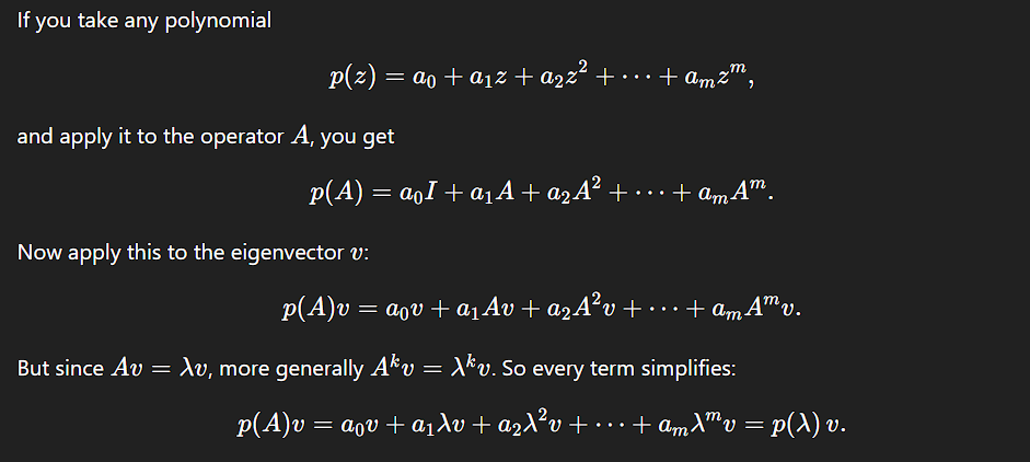
-
Analytic functions (when defined via convergent power series): If converges at , then
Examples: , (when ).
-
Instead of computing (which requires 99 matrix multiplications), if we know the eigendecomposition:
Understanding System Behavior
- Stability: If all , repeated applications of shrink vectors
- Growth: If any , the system exhibits growth
- Oscillations: Complex eigenvalues indicate rotational behavior
Applications
- Principal Component Analysis (PCA): Eigenvectors of covariance matrices
- Google PageRank: Dominant eigenvector of web link matrix
- Quantum Mechanics: Energy states are eigenvalues
- Vibrations: Natural frequencies are related to eigenvalues
Special Cases
Symmetric Matrices
For real symmetric matrices:
- All eigenvalues are real
- Eigenvectors are orthogonal
Diagonal Matrices
Eigenvalues are the diagonal entries, eigenvectors are standard basis vectors
Identity Matrix
Every non-zero vector is an eigenvector with eigenvalue 1
Key Properties
- Trace:
- Determinant:
- Invertibility: is invertible iff all
- Diagonalization: If has independent eigenvectors, then where is diagonal
Sum of Algebraic Multiplicities
For any matrix, the sum of the algebraic multiplicities of all its eigenvalues must equal .
where are the distinct eigenvalues.
The eigenvalues of an matrix are the roots of its characteristic polynomial:
This polynomial will always have degree because:
When expanded, the highest power of comes from the product of diagonal terms:
This gives us plus lower degree terms, so:
By the Fundamental Theorem of Algebra, a polynomial of degree has exactly roots (counting multiplicities) in .
Therefore, the characteristic polynomial has exactly roots, and the sum of their multiplicities must be .
Example
Characteristic polynomial:
- with AM = 2
- with AM = 2
- Sum of multiplicities: ✓
- Real Matrices with Complex Eigenvalues For real matrices, complex eigenvalues come in conjugate pairs: - If is an eigenvalue, so is - Both have the same algebraic multiplicity
Eigendecomposition
Eigendecomposition is the process of breaking down a square matrix into a set of its most fundamental components: its eigenvalues and eigenvectors.
If a matrix is diagonalizable, it can be expressed in the form:
This equation is the eigendecomposition of .
- : The original matrix that we are decomposing
- : An matrix whose columns are the linearly independent eigenvectors of
- : A diagonal matrix containing the eigenvalues of . Each eigenvalue on the diagonal corresponds to the eigenvector in the same column of
- : The inverse of the eigenvector matrix
Visual Representation
The Condition: The Matrix Must Be Diagonalizable
Eigendecomposition is only possible if the matrix is diagonalizable. This means it must have linearly independent eigenvectors to form the invertible matrix .
Quick Check
For every eigenvalue, its algebraic multiplicity must equal its geometric multiplicity.
Examples of Always Diagonalizable Matrices
- Symmetric matrices
- Matrices with distinct eigenvalues
- Orthogonal matrices
Why is Eigendecomposition Useful?
Decomposing a matrix into its eigenvalues and eigenvectors is incredibly useful because it reveals the matrix’s fundamental properties and simplifies complex calculations.
1. It Reveals the Geometry of the Transformation
The formula provides deep insight into what the matrix does to a vector. It says the transformation is equivalent to three simple steps:
- : Change from the standard basis to the basis of eigenvectors
- : Perform a simple scaling along these new eigenvector axes
- : Change back to the standard basis
It shows that even a complex-looking transformation is just a simple stretch/shrink along its special eigenvector directions.
It transforms the matrix from its “standard coordinate” representation into its most natural form—scaling along its eigenvector directions.
2. It Simplifies Calculations
Computing Powers
Instead of multiplying by itself 100 times:
Calculating is trivial—just raise each diagonal eigenvalue to the 100th power:
Matrix Exponential
where
3. Key Applications
Eigendecomposition is a cornerstone of many advanced fields:
| Field | Application |
|---|---|
| Physics | Solving systems of linear differential equations |
| Data Science | Principal Component Analysis (PCA) for dimensionality reduction |
| Quantum Mechanics | Finding the principal states of a system |
| Engineering | Stability analysis of dynamical systems |
| Computer Graphics | Rotation and transformation calculations |
| Machine Learning | Spectral clustering, kernel methods |
Diagonalizable Matrices
A square matrix is diagonalizable if it is similar to a diagonal matrix. This means the matrix can be written as:
where:
- is a diagonal matrix of the eigenvalues
- is an invertible matrix whose columns are the corresponding linearly independent eigenvectors
Conceptually, this means the transformation represented by becomes a simple scaling operation when viewed in a coordinate system defined by its eigenvectors.
Diagonalizing a matrix is like finding a new coordinate system (defined by the eigenvectors) in which the transformation represented by the matrix A is much simpler as it just stretches or shrinks the space along the new coordinate axes (by the amounts of the eigenvalues).
The Test for Diagonalizability
The easiest way to determine if a matrix is diagonalizable is to compare the multiplicities of its eigenvalues. An matrix is diagonalizable if and only if for every eigenvalue :
- Algebraic Multiplicity (AM): How many times an eigenvalue is a root of the characteristic polynomial
- Geometric Multiplicity (GM): The dimension of the eigenspace for that eigenvalue (i.e., the number of linearly independent eigenvectors)
If even one eigenvalue fails this test (GM < AM), the matrix is not diagonalizable.
The Diagonalization Process
Given a diagonalizable matrix :
- Find all eigenvalues by solving
- Find eigenvectors for each eigenvalue by solving
- Form matrix with eigenvectors as columns, by stacking independent eigenvectors as columns.
- Form diagonal matrix with corresponding eigenvalues. The -th diagonal entry matches the eigenvalue of the -th column of .
- Verify:
Examples
Diagonalizable Matrix
Eigenvalues: ,
- : AM = 1, GM = 1 ✓
- : AM = 1, GM = 1 ✓
Conclusion: Diagonalizable!
Non-Diagonalizable Matrix
Eigenvalue: (with AM = 2)
Find eigenspace
Eigenspace: , so GM = 1
Conclusion: GM (1) < AM (2), so not diagonalizable!
-
If an matrix has distinct eigenvalues, it’s automatically diagonalizable.
-
The Spectral Theorem : Real symmetric matrices are always diagonalizable (by orthogonal matrices).
A real symmetric matrix will always have real eigenvalues. This is not true for non-symmetric matrices, which can have complex eigenvalues
  What is an Orthogonal Matrix?

  An orthogonal matrix Q is a special kind of square matrix with the following properties:

  All of its columns (and rows) are orthonormal. This means each column vector has a length of 1, and each column vector is perpendicular (orthogonal) to all other column vectors.
The inverse of an orthogonal matrix is its transpose:
Orthogonal matrices represent transformations that preserve lengths and angles, such as rotations and reflections
The eigenvectors corresponding to distinct eigenvalues of real symmetric matrix are always orthogonal to each other.
The transformation represented by a real symmetric matrix can be understood as a simple scaling (stretching or shrinking) along a set of perpendicular axes. The orthogonal matrix Q represents the rotation needed to align the standard coordinate axes with these new, perpendicular axes (the eigenvectors).
-
An matrix is diagonalizable if and only if it has linearly independent eigenvectors.
Example : Diagonalizing Matrix C
Matrix C
1. Determine if it’s Diagonalizable
Finding Eigenvalues
Solve :
Expanding along the first row:
- First determinant (triangular):
- Second determinant:
Characteristic equation:
This gives:
- (multiplicity 2)
- or
Eigenvalues: , , ,
Checking Geometric Multiplicity for λ = 1
- Rank = 2 (two pivots)
- Geometric multiplicity =
- Algebraic multiplicity = 2
Since AM = GM for all eigenvalues, C is diagonalizable.
Example : Diagonalize Matrix C
Finding Eigenvectors
For λ = 0 (Null space of C):
- From : , ,
- Let , then
- Eigenvector:
For λ = 2 (Null space of C - 2I):
- Solution: , ,
- Eigenvector:
For λ = 1 (Null space of C - I):
- From earlier: , , and are free
- Two eigenvectors: ,
Constructing P and D
Constructing D
Key Principle
The diagonal matrix is formed by placing eigenvalues along the main diagonal. The order must correspond to the order of eigenvectors in .
Why Order Matters
The diagonalization equation expands to:
This is equivalent to the system:
Special Cases
Real Schur Decomposition
For non-diagonalizable matrices, we can still decompose: where is orthogonal and is upper triangular.
Why
If we want to compute , we just multiply by itself:
Now, substitute the diagonalized form for each :
Matrix multiplication is associative, which means we can regroup the parentheses however we like. Let’s regroup them in the middle:
Here comes the magic. A matrix multiplied by its inverse is the identity matrix :
And multiplying any matrix by the identity matrix leaves it unchanged :
Finally, is just :
The pattern continues. Let’s look at :
Regroup in the middle:
The in the middle becomes the identity matrix and vanishes:
For
When you write out , you are writing out one hundred times:
When we regroup, every on the right of a term will be next to a on the left of the next term. All these “inner” pairs will cancel out into identity matrices:
All the pairs become , and multiplying by does nothing. You are left with:
- The from the very beginning
- The from the very end
- One hundred ‘s multiplied together in the middle
Therefore:
The Trace of a Matrix
The trace of a square matrix is the sum of the elements on its main diagonal (top-left to bottom-right).
Definition
For an matrix
the trace is
Example
Properties
- Linearity:
- Scalar multiplication: for any scalar
- Cyclic property: (crucial for many proofs!)
- Eigenvalue sum: (sum of all eigenvalues)
- (cyclic permutation)
The trace of a matrix is an invariant property—it doesn’t change even when the coordinate system is rotated or changed. This is because:
This makes trace particularly useful for describing fundamental properties of systems.
Applications
Data Science and Statistics: Measuring Total Variance
In data analysis, the covariance matrix describes how variables spread out and relate to each other.
Key fact: The trace of the covariance matrix equals the total variance of the dataset.
This is fundamental in:
- Principal Component Analysis (PCA): Finding axes that capture maximum variance
- Dimensionality reduction: Preserving as much total variance as possible
Machine Learning
- Nuclear norm: (used in matrix completion)
- Frobenius norm:
- Regularization: Trace penalties encourage certain matrix structures