Lecture 02 - Image Formation & Spatial Domain Processing

Image formation involves capturing a scene via a camera, influenced by:

Illumination: The light source and its intensity.
Scene: The objects being photographed.
Imaging system: The optics (lens, sensor) that project the scene onto a 2D image plane.

This projection results in a continuous image function f(x, y), where f gives a grey value (or intensity) at each point.

The grey value f(x, y) is thus a product of how much light there is and how reflective the object is at that point.

A monochrome image is described by a function:

f(x, y) = i(x, y) · r(x, y)

where:

i(x, y): Illumination function
r(x, y): Reflectance function
f(x, y): Resultant grey value

Digital grey values are usually within the range [0, 255] or normalized to [0, 1].

Sampling and Quantization

Sampling: Converts continuous spatial domain into a discrete grid.
Quantization: Converts continuous intensity values into discrete levels.

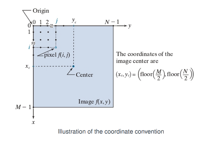
A digital image is a 2D matrix f(x, y) of size M × N (rows × columns).

Each element f(i, j) is a pixel at position (i, j).

Coordinate system:

Origin at the top-left: (0, 0)
Image center: (x_c, y_c) = (⌊M / 2⌋, ⌊N / 2⌋)

alt text

Linear Indexing

Digital images are typically represented as 2D arrays (matrices) where each element corresponds to a pixel intensity. However, in many programming environments or memory storage systems—especially in lower-level languages like C or when interfacing with image files—these 2D arrays are stored in a linear (1D) format in memory.

Computers do not have 2D memory; they store data in a single, long, one-dimensional sequence. To store an image, we must “flatten” its 2D grid of pixels into a 1D list. This process is called linear indexing.

Column-wise scan (column-major order):

alt text

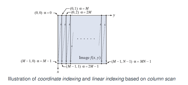
Imagine reading the pixels of the image not like a book (left-to-right, then top-to-bottom), but by going down each column completely before moving to the next column on the right.
As the diagram shows, you start at the top of the first column (y = 0) and go all the way down. Then you move to the top of the second column (y = 1) and go all the way down, and so on.

To convert a 2D coordinate (x, y) to a 1D index α, use the following formula:

α = M · y + x

Where:

M is the number of columns in the image (or matrix).
x is the horizontal coordinate (column index).
y is the vertical coordinate (row index).

Recovery (From 1D index back to 2D coordinates):

x = α mod M
y = (α - x) / M

Column-major order indexing:
This is the order used by Fortran, MATLAB, and OpenCV in some contexts:

α = M · y + x

Where:

M is the number of rows in the matrix.
x is the horizontal coordinate (column index).
y is the vertical coordinate (row index).

→

Row-major order indexing:
This is used in C, C++, Python (NumPy):

α = N · x + y

Where:

N is the number of columns in the matrix.
x is the horizontal coordinate (column index).
y is the vertical coordinate (row index).

Intensity Resolution
Intensity resolution refers to the number of distinct gray levels (or intensity levels) that can be represented in an image.

Bit depth defines the number of bits used to represent the intensity value of each pixel in a digital image. It determines the total number of available tonal (gray) levels that can be encoded.

A b-bit image has 2^b grey levels.

8-bit → 256 levels (0–255)

When too few intensity levels are used for an image that contains smooth gradients (such as a clear sky or a curved surface), an artifact known as posterization or false contouring can appear.

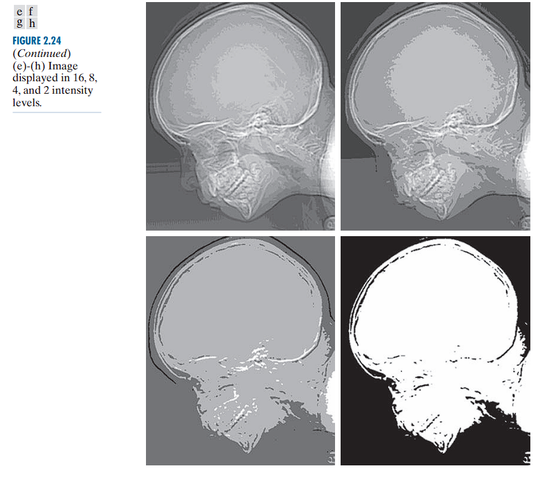
There is a progressive degradation in quality as the number of intensity levels reduces from 256 to 2.

Low resolution (2–16 levels) often reveals unintended contours and artifacts.

alt text

Arithmetic Operations Between Images
Applicable only if the images are of the same size:

Operation	Formula	Meaning
Sum	$s (x, y) = f (x, y) + g (x, y)$	Brightens image or combines intensities
Difference	$d (x, y) = f (x, y) - g (x, y)$	Highlights differences (e.g., motion)
Product	$p (x, y) = f (x, y) \cdot g (x, y)$	Blending, masking
Quotient	$q (x, y) = f (x, y) / g (x, y)$	Contrast normalization

Note: Results can go outside $[0, 255]$ and require post-processing:

Clipping (force into range),
Scaling, or
Rounding to integers.

Noise Reduction by Image Addition

alt text

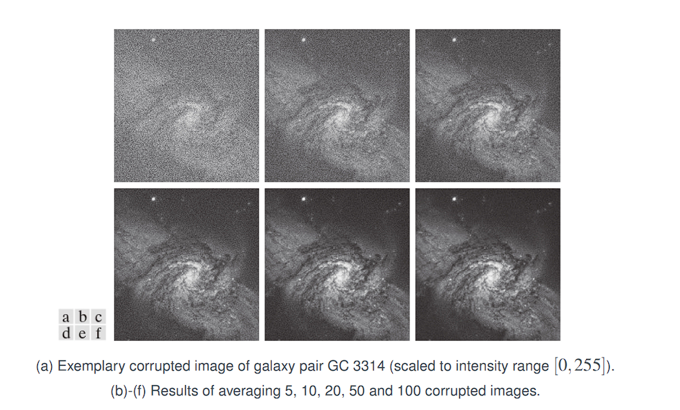
The core idea of this technique is: If you take many photos of the exact same (static) scene, you can average them together to cancel out the random noise, revealing the clean underlying image.

Suppose that g(x, y) is a corrupted image formed by addition of noise η(x, y) to an uncorrupted image f(x, y):

g(x, y) = f(x, y) + η(x, y)

We assume that:

Noise and image values are uncorrelated
This means the amount of noise at a pixel is not related to the pixel’s true brightness. A dark part of the image is just as likely to get a certain random noise value as a bright part.
The noise has zero mean value
For any given pixel, the random noise η is equally likely to be positive (making the pixel brighter) as it is to be negative (making it darker). Over many images, the average of all the random noise values at that one pixel location will be zero:
```
E[η(x, y)] = 0
```

Averaging K noisy images:

$\frac{1}{K} \sum_i = 1^{K} g_{i} (x, y) \approx f (x, y)$

Caution with Differences

Subtraction used to detect changes.

alt text

$g (x, y) = f (x, y) - h (x, y)$

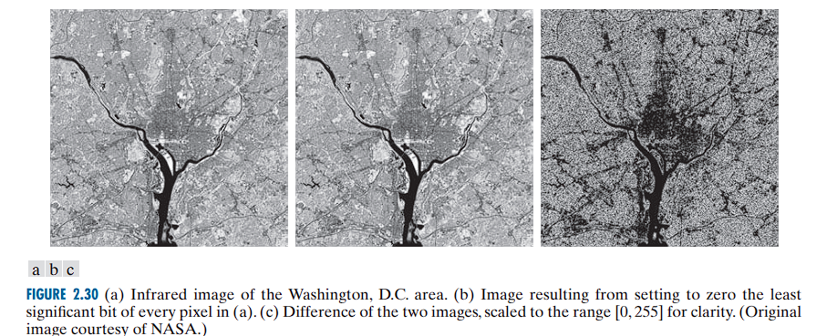
This operation can give negative values.

Problems:

Negative values (which cannot be directly displayed)
Visual indistinguishability unless processed.

When the difference is small, g(x, y) is close to 0, which appears dark or black.
When the difference is large and positive, g(x, y) is a large value, appearing bright or white.

To handle negative results and see the magnitude of the difference, we take the absolute value:

$∣ g (x, y) ∣$

Now, small differences are still dark (near 0) and large differences are bright.

To improve visual interpretability, particularly when differences are small, we invert the image:

$\tilde{g} (x, y) = L - 1 - ∣ g (x, y) ∣$

Where:

L is the intensity resolution, typically 256, so L - 1 = 255.

The effect:

Smaller differences (i.e., areas where the two images are similar) appear brighter (closer to 255).
Larger differences appear darker.

Example
Let us assume:

f(x, y): original image.
h(x, y): same image but with a small object removed (e.g., a person erased).

Compute:

g(x, y) = f(x, y) - h(x, y)

|g(x, y)| gives zero everywhere except where the object was removed.

g̃(x, y) = 255 - |g(x, y)|

Results:

All unchanged areas → g̃ = 255 (white).
Changed area (object removed) → darker pixels (as intensity difference is non-zero).

Visualization:

The resulting image g̃ will appear white everywhere, with dark pixels exactly where the image was altered. This makes the change easily detectable by the human eye.

Spatial Domain Processing

The spatial domain refers to the image plane itself.
Image processing methods in this category are based on direct manipulation of pixels.

There are two principal categories of spatial domain processing:

Intensity Transformations
Operate on individual pixels of an image.
Used for tasks such as:
- Contrast manipulation
- Image thresholding
Spatial Filtering
Operates on the neighborhood of every pixel.
Common examples:
- Image smoothing
- Image sharpening

Spatial domain techniques operate directly on the pixel values of an image,
in contrast to frequency domain techniques, which operate on the Fourier transform of the image.

General Formulation of Intensity Transformations:

g(x, y) = T(f(x, y))

Let f(x, y) be the input image and g(x, y) the output image.
Let T be an operator defined over a neighborhood of the point (x, y).

The operator T can be:

Applied to the pixels of a single image or
Applied to a set of images, such as computing the element-wise sum across multiple images (e.g., for noise reduction).

Example: Local Averaging

Suppose the neighborhood is a square of size 3 × 3, and the operator T is defined as:

Compute the average intensity of all pixels in the neighborhood.

At an arbitrary pixel location, say (100, 150), the result at that location in the output image g(100, 150) is computed as:

g(100, 150) = (1/9) × [sum of f(100, 150) and its 8 neighbors]

The center of the neighborhood is then moved to the next pixel, and the operation is repeated to compute the full output image g(x, y).

Special Case: 1×1 Neighborhood

The smallest possible neighborhood is 1 × 1. In this case, the output g(x, y) depends only on the value of the input image f(x, y) at the same location.
The transformation becomes a pointwise intensity transformation, expressed as:

s = T(r)

Where:

r is the intensity of the input image f(x, y)
s is the intensity of the output image g(x, y)

This transformation maps each intensity value r in the input to a new intensity value s in the output.

Point Operations (Intensity Transformations)

These are also known as point processing operations, since each output pixel value depends only on the corresponding input pixel value (i.e., a 1×1 neighborhood).

If T depends only on the pixel itself, it is called a point operation.

Example: Contrast Stretching and Thresholding

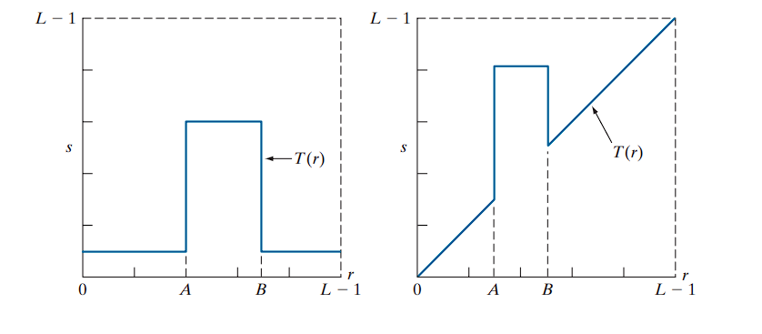
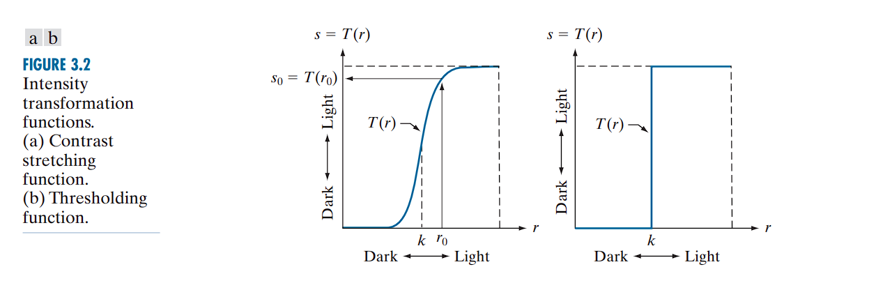alt text If T(r) has the shape shown in a typical contrast-stretching curve (Fig (a)):

Intensities below a threshold k are darkened
Intensities above k are brightened

This enhances image contrast by expanding the range of intensity values.

In the limiting case (as Fig(b)), T(r) becomes a binary threshold function, producing a two-level (black-and-white) image.

Such a transformation is known as a thresholding function.

Neighborhood operations apply a function T over a local region of the image.

Point operations apply T directly to each pixel without considering neighbors.

Image Enhancement

Definition:
Enhancement is the process of manipulating an image so that the result is more suitable than the original for a specific application.

Example:
A method effective for enhancing X-ray images may not be ideal for enhancing infrared images. The choice of enhancement technique depends on the nature of the data and the intended use.

Intensity Transformations

Intensity transformations are pointwise operations, meaning they apply a transformation function to individual pixels, independent of their neighbors.

We use the following notation:

r: Original intensity value of a pixel (input)
s: Transformed intensity value (output)

Both r and s range from 0 to L − 1, where L is the number of intensity levels.
For an 8-bit grayscale image, L = 256 → values in [0, 255].

Transformation Function: `T(r)`

Let T(r) be the transformation function applied to each pixel:

s = T(r)

Where T defines how the input value r is mapped to output s.

Implementation via Lookup Tables (LUT)

Rather than computing T(r) for each pixel in real-time (which is computationally inefficient), intensity transformations are commonly implemented using lookup tables (LUTs).

Steps:

Precompute the values of T(r) for all r in the range [0, 255].
Store these values in a lookup table (an array of 256 entries).
For each pixel in the image:
- Retrieve the original value r.
- Replace it with the transformed value T(r) using the LUT.

This method is both fast and efficient, especially for large images or real-time applications.

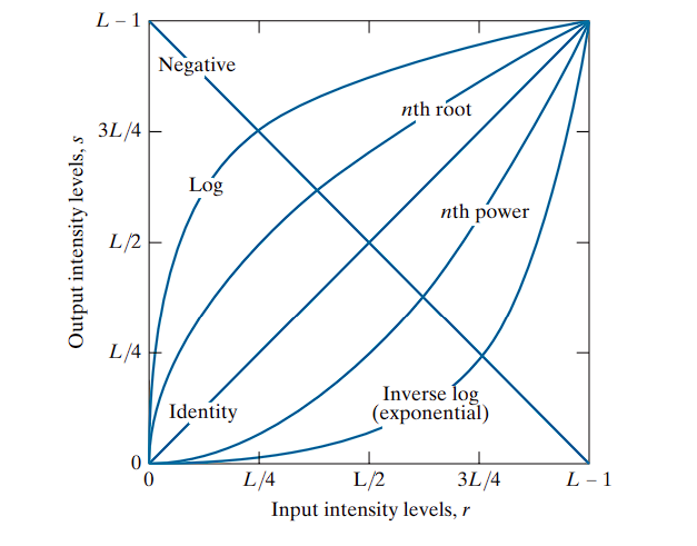
Image Negatives (Negative Transformation)

Definition:
The negative transformation inverts the intensity values of an image by mapping each pixel’s brightness to its opposite within the intensity range.

The transformation function is:

T(r) = L − 1 − r

Where:

r is the original intensity value (input pixel),
T(r) is the transformed intensity (output),
L is the total number of intensity levels (e.g., 256 for 8-bit images).

Effect:

Black becomes white, and white becomes black.
Mid-gray values remain relatively unchanged.
The dynamic range is reversed: the brightest parts become the darkest, and vice versa.

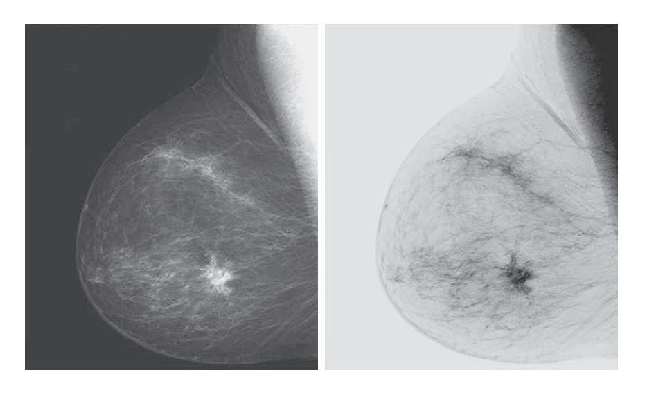
Applications:

Enhancing dark details in images with poor lighting.
Commonly used in:
- Medical imaging, such as X-rays or mammograms,
- Astronomical images to highlight faint stars or nebulae.

Example:

Original intensity value: r = 50
If L = 256, then:

T(50) = 255 − 50 = 205

The pixel becomes much brighter in the negative image.

Logarithmic Transformation

Definition:
The logarithmic transformation enhances the lower intensity values in an image, thereby expanding dark regions and compressing bright ones. It is mathematically defined as:

T(r) = c · log(1 + r)

Where:

r is the input pixel intensity (0 ≤ r ≤ L − 1),
T(r) is the output transformed intensity,
c is a positive constant that scales the result,
log denotes the natural logarithm (or logarithm to base 10, depending on implementation).

Purpose and Effect:

Expands low-intensity values: useful for revealing detail in dark regions.
Compresses high-intensity values: bright areas are mapped to a smaller range.
Particularly effective when the image’s histogram is skewed toward lower intensities.

Mapping Characteristics:

Input levels in the range [0, L/4] are stretched across a wider output range, say [0, 3L/4].
Conversely, input levels in [L/4, L − 1] are compressed into a narrower output range.

This means the transformation emphasizes differences in dark tones while reducing contrast in bright regions.

Constant `c`:

Chosen such that the output remains within the allowable intensity range [0, L − 1].
Typically computed as:

c = (L − 1) / log(1 + R_max)

Where R_max is the maximum possible input intensity value (e.g., 255 for 8-bit images).

Inverse Transformation (Exponential):

To achieve the opposite effect (i.e., compressing dark values and expanding bright values), an exponential transformation is used:

T(r) = c · (e^r − 1)

This is useful when bright regions contain the most important information.

The logarithmic function is valuable in image processing because it compresses the dynamic range of pixel intensity values.

Dynamic Range

Dynamic range refers to the ratio between the maximum and minimum values in a dataset.
In the context of images, it is the range between the darkest pixel and the brightest pixel.

Example:

An image of a Fourier spectrum might contain intensity values ranging from 0 to 1,000,000 or more.
However, most displays (e.g., monitors) and the human visual system can only handle 8-bit intensity levels, i.e., 256 discrete values ranging from 0 to 255.

If you use a simple linear mapping to display such high-dynamic-range images:

The maximum value (e.g., 1,000,000) is mapped to 255 (white).
A moderately high value like 100,000 gets mapped to ~25.
A value of 1,000 is mapped to ~0 (black).

This leads to a loss of detail in most of the image, as many values collapse into the darkest levels (black).

The logarithmic transformation scales intensity values according to:

T(r) = c · log(1 + r)

This transformation maps large input values into a compressed output range:

log(1,000,000) ≈ 6
log(1,000) ≈ 3
log(10) ≈ 1

So, instead of mapping from 0–1,000,000 linearly into 0–255, the log function reduces the effective range, preserving relative differences even in high-intensity regions.

Effect:

Maintains visual detail in bright regions.
Makes the output image more interpretable and displayable.
Especially useful in scientific imaging, e.g., Fourier spectra, astronomy, or medical imaging.

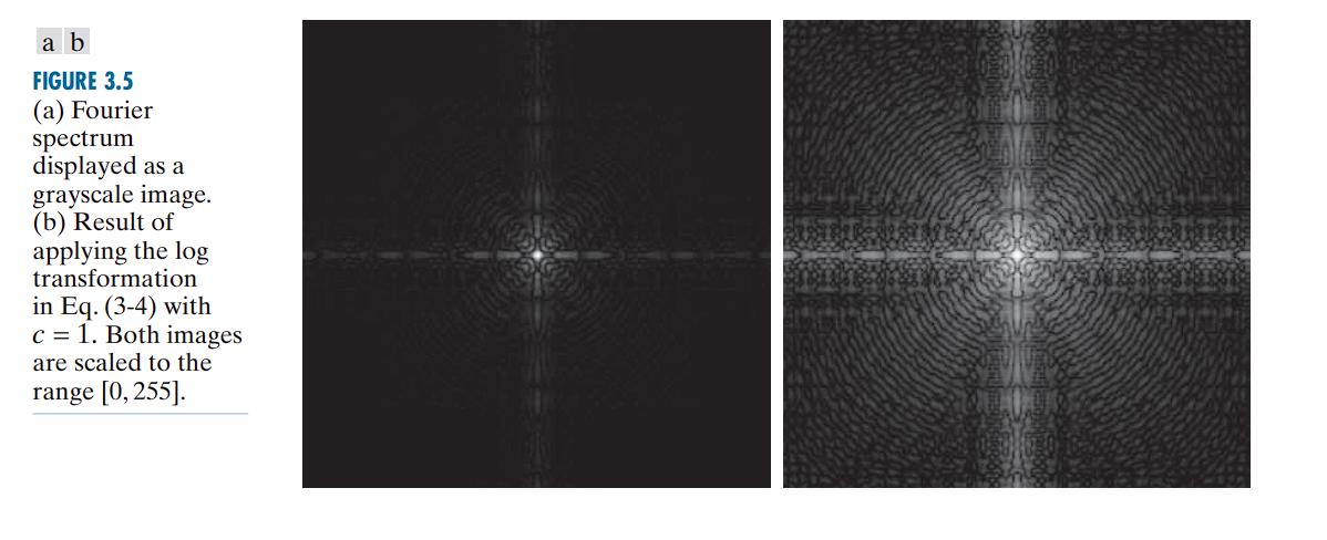
The Fourier Spectrum Example:

Without log transform: You see a few bright white dots against a completely black background. All the important but less intense structural detail is invisible.

With log transform: The intensely bright values are “toned down” significantly, while the fainter (but still important) values are brightened relative to them. Suddenly, you can see all the intricate patterns of the spectrum that were previously hidden.

alt text

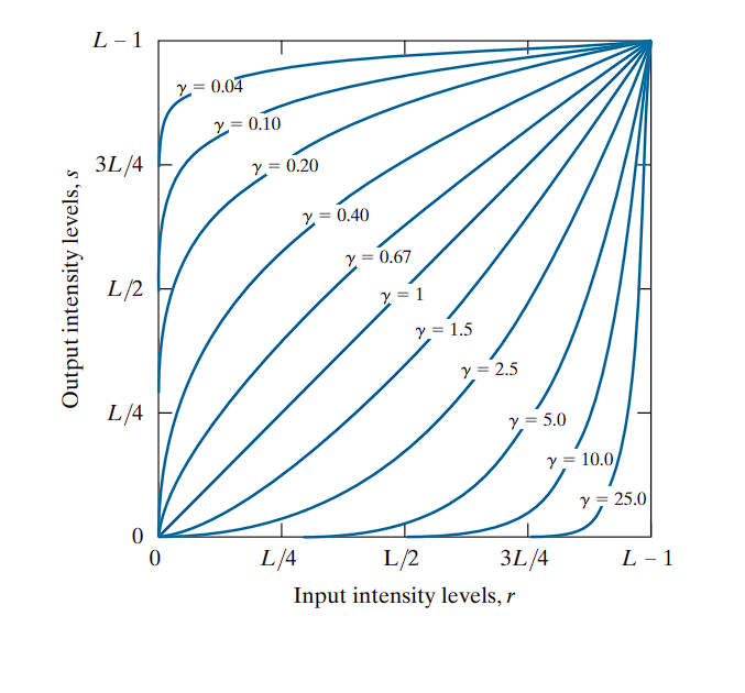
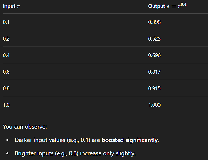
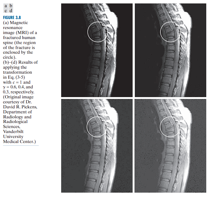
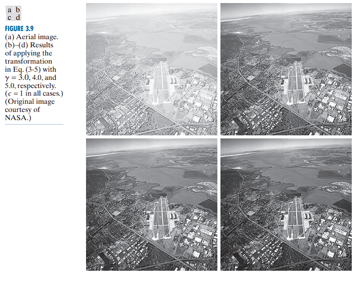
Power-Law (Gamma) Transformations

Power-law transformations are defined as:

$T (r) = c \cdot r^{γ}$

Where:

r: Input pixel intensity (normalized between 0 and 1).
T(r): Output pixel intensity.
c: A positive constant for scaling (commonly set to 1).
γ (gamma): The exponent that controls the transformation behavior.

Behavior Based on Gamma (γ)

γ < 1:
- Expands dark tones.
- Compresses bright tones.
- Useful for enhancing details in dark regions.
γ > 1:
- Compresses dark tones.
- Expands bright tones.
- Useful for brightening already bright areas and suppressing dark ones.

Gamma Correction is widely used in display systems (e.g., TVs, monitors, cameras).
- Most displays apply a γ > 1 transformation to match the nonlinear perception of brightness by the human eye.
- Cameras often apply an inverse gamma to linearize recorded images.
An extended version of the transformation may include an offset:

s = c \cdot (r + ε)^{γ}

This accounts for non-zero output even when the input is zero ( r = 0).
However, such offsets are typically considered calibration artifacts and are usually ignored in standard formulations.
Both log and power-law transformations serve to compress or expand intensity ranges.
γ < 1 (fractional exponents) have a similar effect to log functions:
- They map dark input values to a wider output range.
- They compress the bright input values.
Conversely, γ > 1 performs the opposite:
- Maps bright input values to a wider range.
- Compresses dark regions.

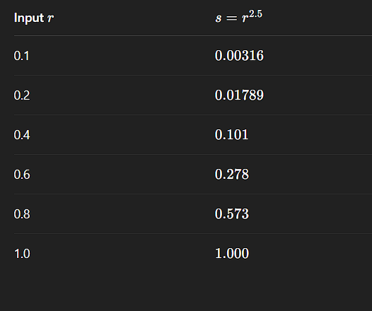
Gamma Correction and Power-Law Response in Imaging Devices

Many electronic imaging devices—such as older CRT monitors, scanners, and certain printers—do not reproduce brightness in a linear manner. Instead, their input-output intensity relationships follow a power-law behavior.

Device Response: Power-Law Nonlinearity

Most display and capture systems obey a response curve of the form:

Output = Input^{γ}

Where:

Input is the normalized signal intensity (0 to 1),
γ (gamma) is the device’s nonlinear response exponent,
Output is the actual intensity produced by the device.

Examples of Gamma Behavior

CRT Monitors typically have a gamma between 1.8 and 2.5.
If an image is not pre-corrected, it appears darker than intended because all dark values are suppressed.
This means:
- If you send a 50% gray signal (Input = 0.5),
- The displayed brightness may only be approximately 0.5²⋅⁵ ≈ 0.18, or 18% of the maximum intensity.
Thus, mid-tones appear darker than intended.

Problem: Visual Distortion

This nonlinear behavior introduces visible distortions, particularly in mid-tone regions:

The image appears too dark on devices with γ > 1.
Linear content (e.g., raw sensor data or computed image outputs) does not render accurately without correction.

Solution: Gamma Correction

To compensate for the device’s distortion, we apply a pre-correction using the inverse gamma function:

Gamma Correction Formula

Corrected Input = Original Input^{1/ γ}

Where:

Original Input: Linear intensity value from the source image,
γ: Gamma of the target display device (e.g., 2.5),
1/γ: Inverse gamma exponent used for pre-correction.

Example:

Suppose a CRT display has a gamma of 2.5.
To correct for this, the image data must be transformed using:

Corrected Input = (Original Input)^{1/2.5} \approx (Original Input)^{0.4}

This brightens the image preemptively, such that when the CRT applies its natural gamma response (darkening), the final result appears visually accurate.

In addition to gamma correction, power-law transformations are useful for general-purpose contrast manipulation. Image enhancement is a balancing act. There is no single “magic” gamma value that works for every image.

γ < 1 brightens an image by mapping dark input values to a wider range of output values

alt text

γ > 1 darkens an image by mapping bright input values to a wider range.

alt text

Piecewise Linear Transformation Functions

In contrast to predefined, smooth transformation curves (such as logarithmic or power-law functions), piecewise linear transformation functions offer highly customizable control over the intensity mapping process.

Piecewise linear transformations divide the input intensity range into multiple segments, within each of which a linear transformation is applied independently.

This allows for:

Arbitrary manipulation of specific intensity ranges.
Local contrast enhancement or suppression.
Fine-grained control over tone curves for applications like contrast enhancement, histogram modification, or tone mapping.

Example Use Case

Suppose the desired behavior is as follows:

Intensity Range	Desired Effect
0 – 50	Brighten the darkest grays significantly.
51 – 180	Leave unchanged (linear mapping, identity).
181 – 255	Slightly darken the brightest values.

A single log or gamma curve cannot achieve this, as they apply a smooth and continuous global transformation. However, a piecewise linear function allows precise control by defining separate linear segments for each region.

To construct such a piecewise function, one needs to define control points ( (r_k, s_k) ), where:

( r_k ): input intensity values (independent variable),
( s_k ): corresponding output intensity values (dependent variable),
The full transformation is a set of linear equations connecting these points.

For example:

Segment 1: ( r = 0 ) to ( r = 50 ) → map to a steeper increase, e.g., ( s = 2r ),
Segment 2: ( r = 51 ) to ( r = 180 ) → identity mapping: ( s = r ),
Segment 3: ( r = 181 ) to ( r = 255 ) → gentle compression: ( s = 0.8r + b ), where ( b ) adjusts for continuity.

This method provides complete control over the transformation curve, making it suitable for highly specific adjustments.

Main Disadvantage: User-Defined Complexity

Transformation Type	User Effort
Power-law transformation	Minimal: Only requires gamma and a scaling constant ( c ).
Piecewise linear	High: Requires explicit definition of control points (r_1, s_1), (r_2, s_2)

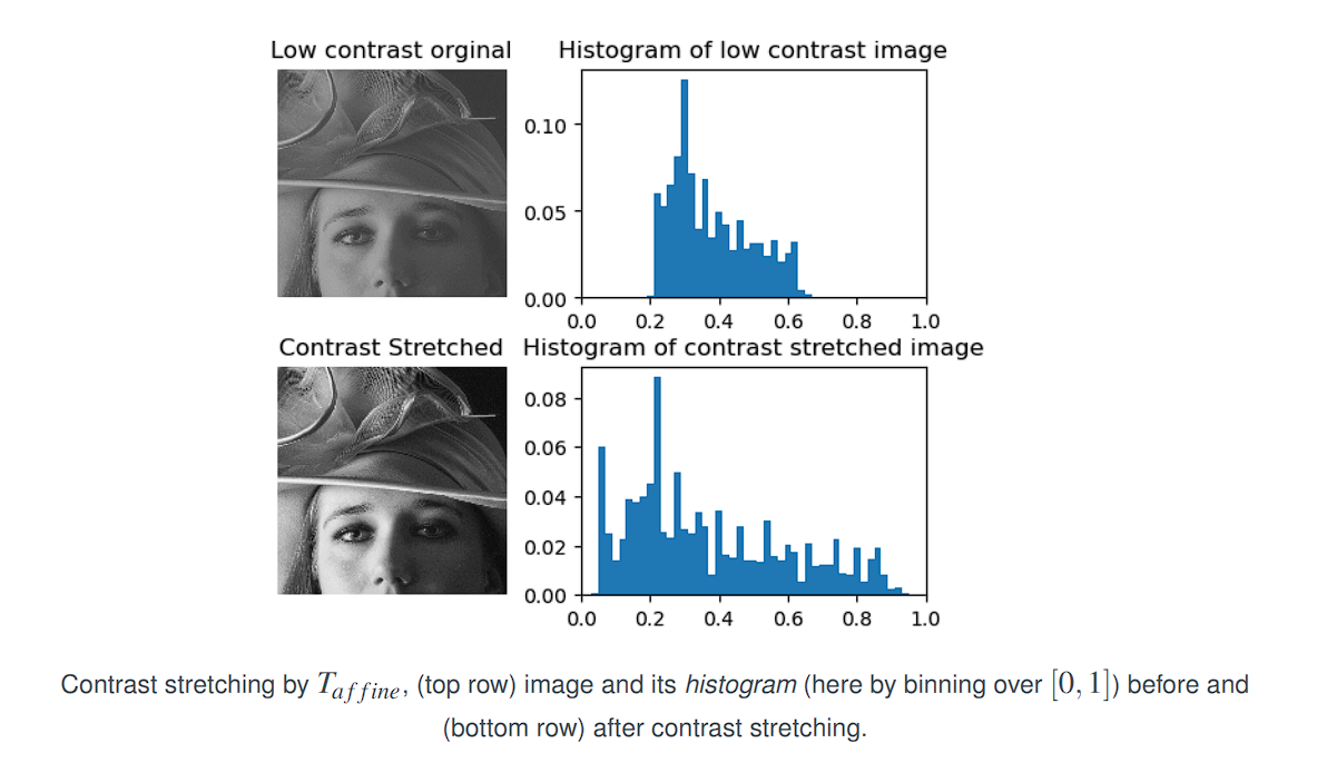
Contrast Stretching

Low-contrast images are often the result of:

Poor illumination conditions,
Limited dynamic range in sensors,
Incorrect acquisition settings (e.g., lens aperture).

Purpose

Linear contrast stretching (also called normalization) is a point-wise intensity transformation used to improve the contrast of a grayscale image by expanding the range of intensity values (gray levels) to span the full available range [0,L−1], where 𝐿 is typically 256 for 8-bit images.

Transformation Function

Let:

( (r_1, s_1) ) and ( (r_2, s_2) ) be user-defined control points,
The transformation function is linear between those points,
Beyond these points, output values may be clipped or scaled accordingly.

Cases:

If ( r_1 = s_1 ) and ( r_2 = s_2 ), the transformation is identity: no change.
If ( r_1 = r_2 ), ( s_1 = 0 ), and ( s_2 = L - 1 ), the function becomes a binary threshold, producing a two-level (black/white) image.
For intermediate values, contrast is enhanced in the selected regions.

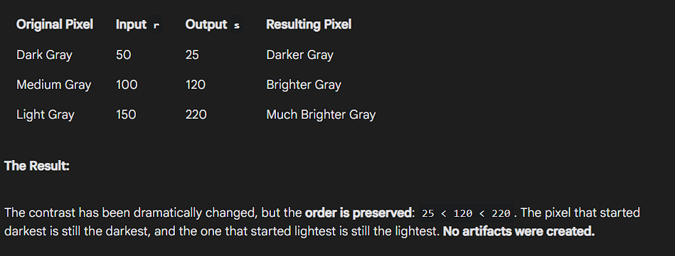
Monotonicity and Artifacts

Artifacts are any unwanted or unnatural visual elements created by a processing step, what happens when you break the monotonicity rule.

To avoid creating artifacts or reordering pixel intensities, the transformation should be:

Single-valued, and
Monotonically increasing, i.e., r₁ ≤ r₂ and s₁ ≤ s₂

Practical Application

Given an 8-bit image:

Let r_min and r_max be the minimum and maximum intensity values in the input image.

To stretch the entire intensity range:

Define:
(r₁, s₁) = (r_min, 0)
(r₂, s₂) = (r_max, L − 1)

This linearly maps the input intensities to span the full range [0, L − 1], improving visual contrast.

The Transformation Function

We define:

r1 = f_min
r2 = f_max
s1 = 0
s2 = L - 1

Then the affine (linear) transformation function is:

T_{affine} (r) = \frac{( r - f _{min} ) ( L - 1 )}{f _{max} - f _{min}}

This maps the original range [f_min, f_max] linearly to [0, L - 1].

Why This Works (Verification)

To verify the correctness of the formula, check its behavior at the boundary values:

Case 1: When r = f_min

T_{affine} (f_{min}) = \frac{( f _{min} - f _{min} ) ( L - 1 )}{f _{max} - f _{min}} = 0 = s_{1}

Case 2: When r = f_max

T_{affine} (f_{max}) = \frac{( f _{max} - f _{min} ) ( L - 1 )}{f _{max} - f _{min}} = L - 1 = s_{2}

Hence, the transformation maps the range [f_min, f_max] to [0, L - 1].

Linear contrast stretching is a pointwise operation that linearly maps the smallest and largest intensity values of the original image to the full display range.

It is particularly effective for enhancing low-contrast images.

alt text

Thresholding Example (Binary Output)

To convert a grayscale image to binary using mean intensity m as a threshold:

Define:
(r₁, s₁) = (m, 0)
(r₂, s₂) = (m, L − 1)

This produces a binary image where:

Intensities < m are mapped to black
Intensities ≥ m are mapped to white

Intensity-Level Slicing

Intensity-level slicing is used to highlight specific ranges of intensity values in an image, often for feature enhancement. This technique is especially useful in applications like:

Enhancing masses of water in satellite imagery
Highlighting flaws or abnormalities in X-ray images

There are two primary approaches:

1. Binary Slicing

Definition: Map the intensities within a specified range to one fixed value (e.g., white), and all other intensities to another value (e.g., black).
Effect: Produces a binary image.
Use Case: When only the presence or absence of a particular intensity range is important.

Example:

If the range of interest is from A to B, then:

For all r such that A ≤ r ≤ B, map to 255 (white)
Otherwise, map to 0 (black)

2. Slicing with Background Retained

Definition: Brighten or darken the intensity values within a specified range, but leave all other intensities unchanged.
Effect: Preserves the original image, while emphasizing a particular range.
Use Case: Useful when it is important to both highlight certain regions and maintain the context provided by the rest of the image.

Bit-Plane Slicing

Bit-Plane Slicing is a technique that decomposes an image into its constituent binary bit planes, highlighting the contribution of each bit to the overall image appearance.

An 8-bit image uses 8 bits to represent each pixel, allowing for 2⁸ = 256 intensity levels (0-255).

Bit Planes:
An 8-bit image can be viewed as consisting of eight separate binary images (bit planes).
- Plane 1 contains the lowest-order bit (least significant bit) of all pixels.
- Plane 8 contains the highest-order bit (most significant bit).

alt text

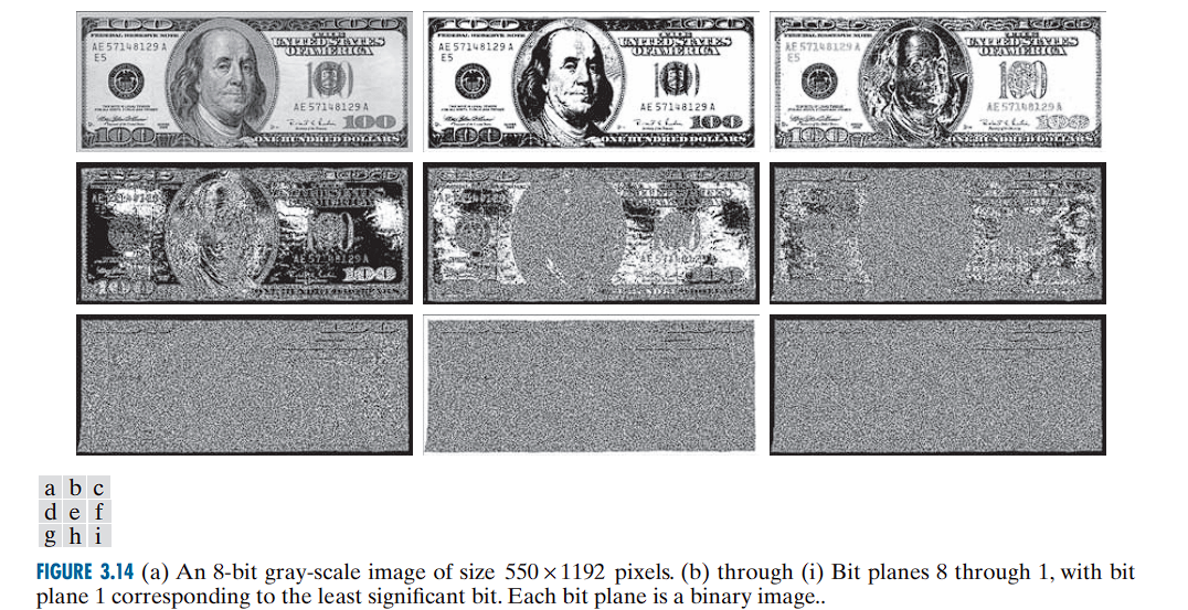
Observations

The higher-order bit planes (especially bits 8 and 7) contain most of the visually significant data.
Lower-order bit planes contribute finer intensity details and subtle textures.

Example of Pixel Bit Values

Consider a pixel with intensity 194:

Its binary representation is: 1 1 0 0 0 0 1 0 (from bit 8 to bit 1).
Corresponding pixels in each bit plane represent these binary bits.
The 8th bit (Most Significant Bit, MSB) is 1.
The 7th bit is 1.
The 6th bit is 0.
…and so on, down to the 1st bit (Least Significant Bit, LSB), which is 0.

High-Order Bit Planes (e.g., Planes 8 and 7): These contain the most visually significant information. They look like a crude but recognizable version of the original image because the most significant bits define the major shapes and overall brightness areas (e.g., is a pixel in the dark half or the light half of the intensity range?).

Low-Order Bit Planes (e.g., Planes 1 and 2): These planes look almost like random noise. They contribute the fine-grained details and subtle texture to the image. A change in the LSB only changes a pixel’s final value by 1, which is often an imperceptible difference.

Generating Bit Planes

The binary image for the 8th bit plane can be generated by thresholding the original image:
- Map intensities in the range ([0, 127]) to 0,
- Map intensities in the range ([128, 255]) to 1.
Similar thresholding functions can be designed for other bit planes

Applications

Image Analysis:
Identifies the importance of each bit in representing image details.
Image Compression:
Often, fewer bit planes than the total are sufficient to reconstruct an acceptable approximation of the original image.
For example, reconstructing using only bit planes 8 and 7 provides a rough approximation with four intensity levels.

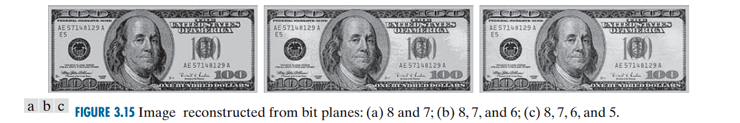
Reconstruction Example

The reconstruction from selected bit planes is performed by multiplying the bit plane n by 2^{n-1} and summing across planes.
For instance:
$Reconstructed Image = (Plane 8 \times 128) + (Plane 7 \times 64) + \dots$
- Using only planes 8 and 7 yields a flat image with four intensity levels.
  - You only have two bits of information, which can only produce 2² = 4 distinct gray levels (0, 64, 128, and 192).
  - Result: The main features are visible, but the image looks “flat” and lacks detail because of the severely limited number of gray levels.
- Adding plane 6 reduces flatness but introduces false contouring.
  - Now you have three bits, allowing for 2³ = 8 gray levels.
  - Result: The image looks better, but it suffers from false contouring. This is when smooth gradients of color or brightness are replaced with visible, sharp steps, like the contour lines on a topographic map.
- Including plane 5 further improves quality and reduces contouring artifacts.
  - With four bits, you have 2⁴ = 16 gray levels.
Using the four highest-order bit planes can reconstruct the image with acceptable detail, while reducing storage by approximately 50%.

Common Point Operations

alt text

Agney's Digital Garden

📁 Explorer

Lecture 02 - Image Formation & Spatial Domain Processing

Noise Reduction by Image Addition

Caution with Differences

Spatial Domain Processing

Example: Local Averaging

Special Case: 1×1 Neighborhood

Point Operations (Intensity Transformations)

Example: Contrast Stretching and Thresholding

Image Enhancement

Intensity Transformations

Transformation Function: T(r)

Implementation via Lookup Tables (LUT)

Steps:

Image Negatives (Negative Transformation)

Effect:

Applications:

Example:

Logarithmic Transformation

Purpose and Effect:

Mapping Characteristics:

Constant c:

Inverse Transformation (Exponential):

Effect:

The Fourier Spectrum Example:

Power-Law (Gamma) Transformations

Behavior Based on Gamma (γ)

Gamma Correction and Power-Law Response in Imaging Devices

Device Response: Power-Law Nonlinearity

Examples of Gamma Behavior

Problem: Visual Distortion

Solution: Gamma Correction

Gamma Correction Formula

γ < 1 brightens an image by mapping dark input values to a wider range of output values

γ > 1 darkens an image by mapping bright input values to a wider range.

Piecewise Linear Transformation Functions

Example Use Case

For example:

Main Disadvantage: User-Defined Complexity

Contrast Stretching

Purpose

Transformation Function

Monotonicity and Artifacts

Practical Application

The Transformation Function

Why This Works (Verification)

Thresholding Example (Binary Output)

Intensity-Level Slicing

1. Binary Slicing

2. Slicing with Background Retained

Bit-Plane Slicing

Observations

Example of Pixel Bit Values

Generating Bit Planes

Applications

Reconstruction Example

Common Point Operations

Graph View

Table of Contents

Backlinks

Transformation Function: `T(r)`

Constant `c`: