Lecture 03 - Histograms & Histogram Equalization

Image Histogram

An image histogram is a fundamental tool used for analyzing and manipulating digital images. It provides a graphical representation of the distribution of pixel intensity values.

---

Definitions

• Image Size (M, N):
  An image is a grid of pixels with M rows (height) and N columns (width).

  • Total number of pixels: M × N

• Grey Values (r_k, L):
  Brightness is quantized into discrete levels.

  • L: Number of grey levels (e.g., L = 256 for 8-bit images)
  • r_k: A grey level, where r_0 = 0 (black), r_{L-1} = 255 (white)

• Pixel Count (n_k):
  The number of pixels in the image having grey level r_k.

  • For example, n_0 is the count of pixels with intensity 0.

• Unnormalized Histogram h(r_k):
  The raw count of pixels for each grey level.
  h(r_k) = n_k

  • Depends on image size
  • Not suitable for comparison across different image sizes

• Histogram Bins:
  Each grey level r_k is treated as a bin. The histogram distributes pixel values into these L bins.

• Normalized Histogram p(r_k):
  The probability distribution of grey levels across the image:
  p(r_k) = n_k / (M × N)

  • Values lie in [0, 1]
  • Independent of image size
  • The sum of all p(r_k) is 1

---

Numerical Example

A 4×4 grayscale image with ( L = 8 ) grey levels:

[ 2, 3, 3, 4 ]
[ 1, 2, 4, 5 ]
[ 0, 1, 5, 6 ]
[ 1, 2, 6, 7 ]

• Rows: M = 4
• Columns: N = 4
• Total pixels: M × N = 16
• Grey levels: r_k ∈ {0, 1, ..., 7}

Step 2: Unnormalized Histogram

( r_k )	( n_k )
0	1
1	3
2	3
3	2
4	2
5	2
6	2
7	1
Total	16

Step 3: Normalized Histogram p(r_k) = n_k / 16

Grey Value r_k	Count n_k	Normalized p(r_k)
0	1	1/16 = 0.0625
1	3	3/16 = 0.1875
2	3	3/16 = 0.1875
3	2	2/16 = 0.125
4	2	2/16 = 0.125
5	2	2/16 = 0.125
6	2	2/16 = 0.125
7	1	1/16 = 0.0625
Total	16	1.0

---

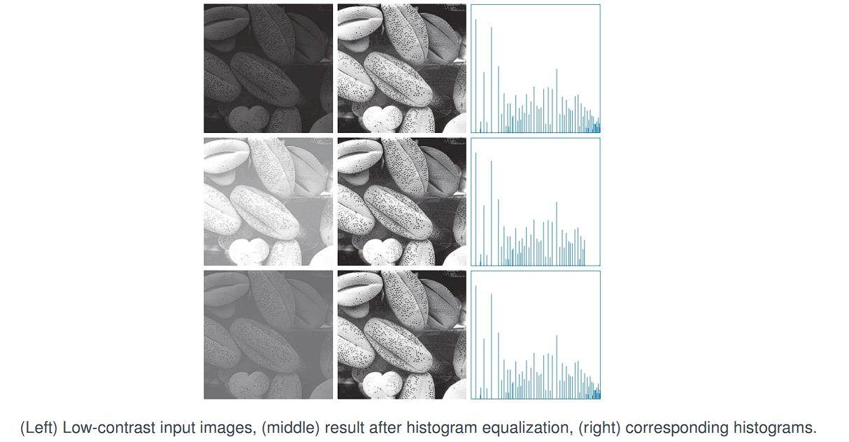
Histogram Equalization

The goal of histogram equalization is to find a transformation function s = T(r) that takes an input image with any kind of histogram and produces an output image whose histogram is perfectly flat (uniform).

We treat intensity values r ∈ [0, L−1] as continuous variables, and define a transformation:

s = T(r)

---

Key Requirement

• T(r) must be monotonically increasing to preserve intensity ordering.
• Strict monotonicity ensures a one-to-one mapping from input to output values.

---

Transformation Function

$$s=T(r)=(L-1){\int }_0^r{p}_r(\alpha )d\alpha$$

Where:

• p_r(r) is the probability density function (PDF) of the original image (i.e., the normalized histogram).
• The integral accumulates the probability from 0 to r, which is the cumulative distribution function (CDF).
• The output s lies within [0, L−1].

---

Result

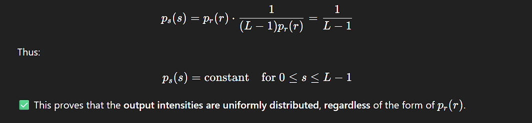
After applying the transformation T(r), the new intensity distribution p_s(s) becomes uniform:

p_s(s) = 1    for 0 ≤ s ≤ L − 1

This implies that the histogram of the output image is flattened (equalized), leading to enhanced contrast.

p_r(r) is the histogram (or PDF) of the original image with intensities r.

p_s(s) is the histogram (or PDF) of the new, transformed image with intensities s.

---

Inverse Transformation

In some formulations, we apply the inverse transformation:

r = T⁻¹(s)    for 0 ≤ s ≤ L − 1

To ensure this works properly, we modify the conditions:

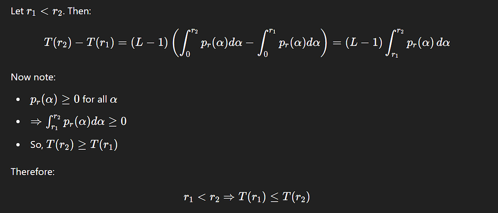
• T(r) must be a strictly monotonic increasing function in the interval 0 ≤ r ≤ L − 1

---

Monotonic vs. Strictly Monotonic Transformations

• T(r) is monotonic increasing, meaning:

  T(r₂) ≥ T(r₁) for r₂ > r₁
  

• However, multiple input values may map to a single output value (i.e., many-to-one mapping).
• This is acceptable for forward mapping (r → s) but problematic for inverse mapping, as not all output values s can uniquely determine their input r.

By requiring that T(r) be strictly monotonic:

• Strict monotonicity:

  T(r₂) > T(r₁) for r₂ > r₁
  

• Guarantees a one-to-one mapping both forward and backward (r ↔ s).

---

Let:

• r and s be random variables representing input and output intensity values.
• p_r(r) and p_s(s) be the probability density functions (PDFs) for r and s.

If:

• T(r) is continuous and differentiable,
• and we know p_r(r) and T(r),

Then the output PDF p_s(s) is given by:

$$p_s(s)=p_r(r)\ast (dr/ds)$$

---

Deriving p_s(s) from p_r(r)

Using Leibniz’s Rule:

ds/dr = dT(r)/dr = (L − 1) * p_r(r)

Therefore:

dr/ds = 1 / [(L − 1) * p_r(r)]

Substitute into
p_s(s) = p_r(r) * (dr/ds)

---

---

Spatial Filtering

Spatial filtering involves modifying an image by applying a function to the neighborhood of each pixel. The process replaces each pixel’s value with a new value computed from its surroundings.

The term filter originates from frequency domain processing, where filtering refers to the process of passing, modifying, or suppressing specific frequency components within an image. For instance:

• A lowpass filter allows low-frequency components to pass while attenuating high frequencies.
• The visual result of applying a lowpass filter is image smoothing, commonly perceived as blurring.

Although frequency domain techniques are a powerful tool for image processing, similar effects—such as smoothing—can also be achieved directly in the spatial domain using spatial filters.

The key idea is to apply a kernel (or mask) over the image, processing each pixel in context with its neighborhood to achieve the desired transformation—such as enhancement, noise reduction, or edge detection.

---

Linear Spatial Filtering

A linear spatial filter operates by performing a sum-of-products between an image f(x, y) and a filter kernel w(s, t). The kernel—also referred to as a mask, template, or window—is a small matrix that defines both:

• The neighborhood over which the filtering is applied, and
• The coefficients that determine the nature of the filtering operation (e.g., smoothing, sharpening).

---

Basic Operation

The mechanics of linear spatial filtering are illustrated using a 3 × 3 kernel. For any pixel at location (x, y) in the input image, the filtered response g(x, y) is given by the sum of products between the kernel coefficients and the corresponding pixels in the neighborhood:

g(x, y) =
    w(-1, -1)·f(x-1, y-1) + w(-1, 0)·f(x-1, y) + w(-1, 1)·f(x-1, y+1) +
    w( 0, -1)·f(x,   y-1) + w( 0, 0)·f(x,   y) + w( 0, 1)·f(x,   y+1) +
    w( 1, -1)·f(x+1, y-1) + w( 1, 0)·f(x+1, y) + w( 1, 1)·f(x+1, y+1)

This represents a typical convolution-like filtering operation.

---

General Form

To generalize for a kernel of size m × n, where m = 2a + 1 and n = 2b + 1 (ensuring odd dimensions), the linear filtering operation is expressed as:

$$g(x,y)={\Sigma }_{s=-a}^a{\Sigma }_{t=-b}^{b}w(s,t)\cdot f(x+s,y+t)$$

This defines the linear filtering process over the entire image.

• f(x + s, y + t) are the neighboring pixels of the input image,
• w(s, t) are the kernel weights, and
• g(x, y) is the corresponding output pixel in the filtered image.

As the coordinates (x, y) are varied across the image, the kernel slides across each pixel location, computing a new filtered value at every position.

The use of odd-sized kernels ensures a well-defined center.

---

Spatial Correlation and Convolution

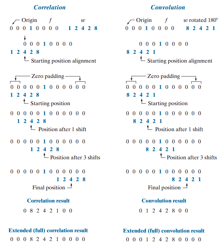
Spatial correlation and spatial convolution are fundamental operations in image processing, both involving a systematic shift of a kernel across an image and computing a sum-of-products at each location. These two operations are nearly identical in execution, with one key difference: convolution requires a 180° rotation of the kernel before the computation.

This distinction becomes meaningful when the kernel is not symmetric about its center. If the kernel is symmetric, both correlation and convolution yield identical results.

---

Step-by-Step Correlation (1D Example)

$$g(x)={\Sigma }_{s=-a}^{a}w(s)\cdot f(x+s)$$

To compute correlation:

1. Initial Position (x = 0):
   Align the center of the kernel with the first position of the input.
   Compute the first value:

   $$g(0)={\Sigma }_{s=-2}^{2}w(s)\cdot f(s)$$

2. Shift Right (x = 1):
   Shift the kernel one position to the right and repeat the sum-of-products.

   $$g(1)={\Sigma }_{s=-2}^{2}w(s)\cdot f(1+s)$$

3. Continue Sliding:
   Repeat this process by incrementing x step by step until the kernel has fully passed over the input signal.

The result is a new signal g(x), where each value represents the correlation output at position x.

---

Full vs. Standard Correlation

• The standard correlation result is generated by starting with the center of the kernel aligned with the image origin and stopping when the kernel’s center passes the last pixel.
• Full correlation extends this by allowing every kernel element to interact with every image element, requiring zero-padding at the boundaries.

Cropping the full correlation result gives the standard correlation output.

---

1. Displacement-Dependent Output:
   Correlation values vary based on how far the kernel is displaced from the origin. Each shift by one unit results in a new correlation value.

2. Response to Unit Impulse:
   If f(x) is a discrete unit impulse (i.e., a sequence of all zeros with a single one), then the correlation result is a 180° rotated copy of the kernel.
   This illustrates that correlation introduces reversal when applied to an impulse.

---

Convolution

In convolution, the only difference is that the kernel is pre-rotated by 180° before applying the same sliding sum-of-products procedure. This pre-rotation ensures that:

• Convolution with a unit impulse yields a direct (non-rotated) copy of the kernel.
• Convolution of a function with an impulse copies the function to the location of the impulse
• This is a foundational result in linear system theory.

Mathematically, convolution in 1D is represented as:

$$g(x)={\Sigma }_{s=-a}^{a}w(-s)\cdot f(x+s)$$

This equation introduces a mirroring of the kernel

---

Correlation and Convolution to 2D Images

Padding and Kernel Placement

The concepts of 1D spatial correlation and convolution extend naturally to 2D image processing. When applying a 2D kernel of size m × n to an image, it is necessary to pad the image boundaries with zeros to allow the kernel to operate on edge pixels.

• The image is padded with:
  • (m - 1) / 2 rows of zeros at the top and bottom, and
  • (n - 1) / 2 columns of zeros on the left and right.

For example, if the kernel size is 3 × 3, one row and one column of zeros are added on each side

---

Correlation on 2D Images

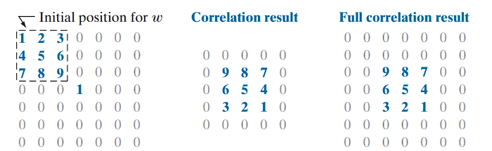
After the kernel has visited every pixel (with its center aligned), the final output is the correlated image. As in the 1D case, the result at the position of a unit impulse is a 180° rotated copy of the kernel.

---

Convolution on 2D Images

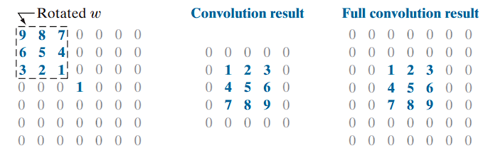
The result of convolving a kernel with an impulse is a direct (non-rotated) copy of the kernel centered at the impulse location.

This behavior reflects a fundamental principle in linear system theory: convolution of a function with a unit impulse produces a copy of that function, shifted to the impulse’s location.

---

Correlation and convolution yield the same result when the kernel is symmetric about its center (i.e., w(i, j) = w(-i, -j) for all i, j).

---

The Discrete Impulse Function

A discrete impulse of strength (or amplitude) A located at coordinates (x₀, y₀) is defined as:

δ(x, y) = {
    A,  if x = x₀ and y = y₀
    0,  otherwise
}

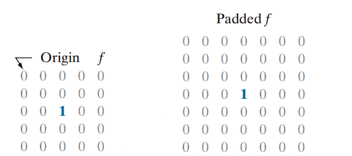
• In the 1D example from Figure 3.29(a), the impulse is represented as δ(x - 3).
• In the 2D example from Figure 3.30(a), the impulse is located at (2, 2), relative to an origin at (0, 0) and is written as δ(x - 2, y - 2).

Every complex image can be broken down into a sum of impulses. Since filters respond predictably to impulses, we can understand how the filter will behave on the entire image by knowing its response to impulses.

A discrete image can be expressed as:

$$f(x,y)=\sum _{(i)}\sum _{(j)}f(i,j)\cdot \delta (x-i,y-j)$$

Where:

• f(x, y): The image function at position (x, y)
• f(i, j): The pixel value at coordinates (i, j)
• δ(x − i, y − j): The 2D discrete unit impulse centered at (i, j)
• The summation runs over all valid pixel coordinates (i, j) in the image domain

Convolving any image f with an impulse δ gives you the original image f back, unchanged. The impulse is to convolution what the number 1 is to multiplication.

f * δ = f

A 5x5 impulse at position (2, 2) would look like this:

[ 0, 0, 0, 0, 0 ]
[ 0, 0, 0, 0, 0 ]
[ 0, 0, 1, 0, 0 ]  <-- The single '1' at (2,2)
[ 0, 0, 0, 0, 0 ]
[ 0, 0, 0, 0, 0 ]

---

Spatial Correlation

The correlation of a kernel w of size m × n with an image f(x, y), denoted as (w ⊗ f)(x, y), is given by:

$$(w\otimes f)(x,y)=\sum _{s=-a}^a\sum _{t=-b}^{b}w(s,t)\cdot f(x+s,y+t)$$

This expression computes the sum of products between the kernel coefficients and the image values centered at (x, y). The process slides the kernel over the entire image, computing this value at every location.

Because our kernels do not depend on (x, y), the notation is often simplified to just w ⊗ f(x, y).

To ensure proper operation at image boundaries, the image f is assumed to be padded appropriately (typically with zeros).

Assuming the kernel dimensions m and n are odd integers, we define:

• a = (m - 1) / 2
• b = (n - 1) / 2

These values represent the number of rows/columns that extend from the center of the kernel in each direction.

---

Spatial Convolution

The convolution of the same kernel w with image f(x, y), denoted as (w * f)(x, y), is defined as:

$$(w\ast f)(x,y)=\sum _{s=-a}^a\sum _{t=-b}^{b}w(s,t)\cdot f(x-s,y-t)$$

Here, the kernel is reflected (rotated by 180°) before performing the same sliding sum-of-products operation. This is achieved mathematically by using the subtraction inside the function arguments f(x - s, y - t).

These minus signs align the coordinates of f and w when one of the functions is rotated 180°

Linear spatial filtering and spatial convolution are synonymous in this context.

Because convolution is commutative, it is immaterial whether w or f is rotated. However, by convention, the kernel w is the one that is rotated prior to performing the convolution operation.

---

Full Correlation and Convolution Coverage

To ensure that every element of a kernel w visits every pixel in an image f, not just its center, the definitions of correlation and convolution can be extended. This requires a modified starting and ending alignment of the kernel with respect to the image.

• Starting alignment: The bottom-right corner of the kernel coincides with the origin of the image.
• Ending alignment: The top-left corner of the kernel coincides with the bottom-right corner of the image.

Padding Requirements

Let:

• w be of size m × n
• f be of size M × N

To support full kernel traversal, the image must be padded with:

• (m - 1) rows: top and bottom
• (n - 1) columns: left and right

Resulting Output Size

With this extended padding, the full correlation or convolution output will have dimensions:

S_v = M + m - 1
S_h = N + n - 1

Thus, the output array will be of size:

S_v × S_h

---

Unlike convolution, correlation is neither commutative nor associative.

Property	Convolution (*)	Correlation (⨂)
Commutative	f * g = g * f	Not generally commutative: f ⨂ g ≠ g ⨂ f
Associative	(f * g) * h = f * (g * h)	Not generally associative
Distributive	f * (g + h) = (f * g) + (f * h)	f ⨂ (g + h) = (f ⨂ g) + (f ⨂ h)

---

Multistage Convolution Filtering

In certain applications, an image is filtered sequentially in multiple stages, where each stage uses a distinct convolution kernel.

For example, let:

• f be the input image
• w₁, w₂, ..., w_Q be a sequence of kernels applied in Q stages

Then the image is processed as follows:

Stage 1:      f₁ = w₁ * f
Stage 2:      f₂ = w₂ * f₁
Stage 3:      f₃ = w₃ * f₂
...
Stage Q:      f_Q = w_Q * f_{Q-1}

However, due to the commutative and associative properties of convolution, this entire process can be replaced by a single convolution:

f_Q = w * f

Where:

w = w₁ * w₂ * w₃ * ... * w_Q

---

Resulting Kernel Size

Let each kernel wₖ have size m × n for all k ∈ [1, Q]. Then, the combined kernel w will have dimensions W_v × W_h, computed as:

Each additional convolution increases the total size by
( m - 1 ) in rows and ( n - 1 ) in columns:

So:

$$W_v=m+(Q-1)(m-1)=Q(m-1)+1\cdot m=Q(m-1)+m$$

W_v = Q × (m - 1)
W_h = Q × (n - 1)

These expressions result from the recursive application of the full convolution dimension formulas:

S_v = M + m - 1
S_h = N + n - 1

These assume that each value of the kernel fully visits the result of the previous convolution stage, using full padding and complete alignment.

---

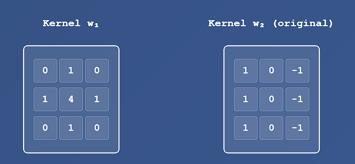
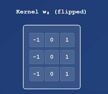
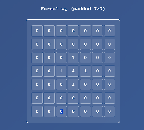
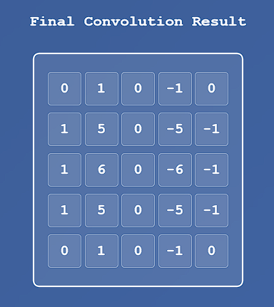
Example : Convolution in 2D of two 3x3 Kernels

---

Separable Spatial Filters

A 2D function G(x, y) is said to be separable if it can be written as the product of two 1D functions:

G(x, y) = G₁(x) · G₂(y)

In image processing, a spatial filter kernel is represented as a matrix. A kernel is said to be separable if it can be expressed as the outer product of two vectors.

Example: Separable Kernel

Consider the following 2 × 3 kernel:

w = [1 1 1
     1 1 1]

This kernel is separable because it can be expressed as:

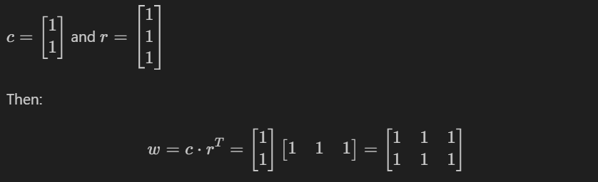
Thus, w is the outer product c · rᵀ.

---

For a separable kernel w of size m × n, it can be written as:

w = v · wᵀ                    

Where:

• v is a column vector of size m × 1
• w is a column vector of size n × 1 (so wᵀ is a 1 × n row vector)

In the special case where the kernel is square, i.e., of size m × m, we can simplify the notation:

w = v · vᵀ                    

The product of a column vector and a row vector yields a matrix. This operation is equivalent to the 2D convolution of the vectors:

w = v * wᵀ

Hence, separable kernels enable more efficient filtering by decomposing a 2D convolution into two 1D convolutions, one along rows and one along columns, significantly reducing computational complexity.

Computational Advantages of Separable Kernels

The primary benefit of using separable kernels lies in the computational efficiency gained through the associative property of convolution.

Suppose we have a kernel w that can be decomposed into two simpler kernels, w₁ and w₂, such that:

w = w₁ * w₂

Then, due to the commutative and associative properties of convolution (see Table 3.5), it follows that:

w * f = (w₁ * w₂) * f = w₁ * (w₂ * f) = w₂ * (w₁ * f)

Let:

• f be an image of size M × N

• w be a filter kernel of size m × n

For Non-Separable Case convolving w with f requires approximately:

O(M · N · m · n)

multiplication and addition operations. This is because every output pixel is influenced by all coefficients in the kernel.

For Separable Case

If w is separable into w₁ (m × 1) and w₂ (1 × n), then:

1. The first convolution, w₁ * f, requires O(M · N · m) operations.
2. The second convolution, w₂ * (w₁ * f), also produces an image of size M × N and requires O(M · N · n) operations.

Thus, the total operations become:

O(M · N · (m + n))

The computational advantage of using a separable kernel versus a non-separable kernel is given by:

C = (M · N · m · n) / (M · N · (m + n)) = (m · n) / (m + n)      

For example, a kernel of size 11 × 11 yields:

C = (11 × 11) / (11 + 11) = 121 / 22 ≈ 5.5

This means filtering can be over five times faster. For large kernels (hundreds of elements), speedups can reach a factor of 100 or more, significantly improving execution time.

---

Determining Kernel Separability

From matrix theory, any matrix formed by the outer product of a column vector and a row vector has rank 1. Since separable kernels are defined in this way, we can determine separability by checking if the kernel matrix has rank 1.

The rank of a matrix is the maximum number of linearly independent rows or columns in the matrix

If rank(w) == 1, then w is separable.

---

Extracting 1D Kernels from a Separable Kernel

To decompose a rank-1 kernel w into its constituent 1D vectors v and wᵀ, follow these steps:

1. Identify a non-zero element in the kernel and denote it as E.
2. Extract the column and row that contain this element. Denote them:
   • c = column vector
   • r = row vector
3. Use the following relationships:

v = c
wᵀ = r / E

Thus:

w = v · wᵀ

This decomposition works because all rows and columns in a rank-1 matrix are linearly dependent—they differ only by scalar multiples.

---

Special Case: Circularly Symmetric Kernels

For circularly symmetric kernels (e.g., Gaussian), the kernel can be described completely by the central column vector. In such cases:

w = v · vᵀ / c

Where:

• v is the central column vector,
• c is the value at the center of the kernel.

Then the 1D components used for convolution become:

w₁ = v
w₂ = vᵀ / c

This allows implementation of the 2D filter using two 1D convolutions, one horizontal and one vertical, maintaining both efficiency and accuracy.

---

Example: Decomposing a Rank-1 Kernel into the Outer Product of Two Vectors

🔷 Given 2D Kernel w

Suppose we are given the following 3 × 3 kernel:

w =
[  2   4   6
   4   8  12
   6  12  18 ]

🔷 Step 1: Pick a Non-Zero Entry

Let’s choose the element at position (0, 0):

E = w[0][0] = 2

---

🔷 Step 2: Extract the Column and Row

Column vector c (first column):

v = [ 2
      4
      6 ]

Row vector r (first row):

r = [ 2  4  6 ]

---

🔷 Step 3: Normalize the Row Vector

To construct the outer product:

v = c
wᵀ = r / E = [ 2/2  4/2  6/2 ] = [ 1  2  3 ]

---

🔷 Final Result

We now have:

v   = [ 2
         4
         6 ]

wᵀ = [ 1  2  3 ]

Taking the outer product:

w = v · wᵀ =
    [ 2×1  2×2  2×3 ]   → [  2   4   6
      4×1  4×2  4×3 ]      4   8  12
      6×1  6×2  6×3 ]      6  12  18 ]

w is separable and equal to the outer product of v and wᵀ.

Example: Decomposition of a Circularly Symmetric Kernel into Separable 1D Components

w = (v · vᵀ) / c

---

🔷 Step 1: Define a Circularly Symmetric Kernel

Consider the following 3×3 Gaussian-like kernel:

w =
[ 1  2  1
  2  4  2
  1  2  1 ]

This kernel is circularly symmetric, as its values are symmetric about the center and decrease radially.

• Center value: c = 4
• Central column vector v (middle column):

v = [ 2
      4
      2 ]

---

🔷 Step 2: Outer Product of v with Itself

Compute the outer product:

v · vᵀ =
[ 2     ]   ·   [ 2  4  2 ] =
[ 4     ]
[ 2     ]

Result:
[  4   8   4
   8  16   8
   4   8   4 ]

---

🔷 Step 3: Normalize by c = 4

Divide the entire matrix by 4:

w = (v · vᵀ) / 4 =
[ 1  2  1
  2  4  2
  1  2  1 ]

This matches the original kernel.

---