Lecture 04 - Spatial Filtering & Convolution

Spatial vs Frequency Domain: The Role of the Fourier Transform

The connection between spatial- and frequency-domain processing is established by the Fourier transform.

• To move from the spatial domain to the frequency domain, we use the Fourier transform.
• To return, we use the inverse Fourier transform.

---

1. Convolution in the spatial domain is equivalent to multiplication in the frequency domain, and vice versa.
2. An impulse of strength A in the spatial domain is a constant value A in the frequency domain, and vice versa.

    δ(x, y) = {
                      A   if x = x₀ and y = y₀
                      0   otherwise
    }

    The 2D **Fourier Transform** of a shifted impulse `δ(x − x₀, y − y₀)` results in a complex exponential. However, when the impulse is **centered at the origin** `(x₀, y₀) = (0, 0)`, the transform is:

                        F{δ(x, y)} = A

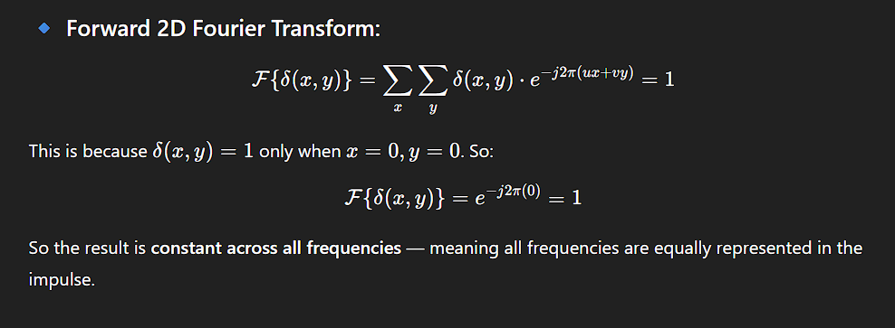
Interpretation:
In the frequency domain, all frequencies are present equally with a constant amplitude A.

Duality Summary:

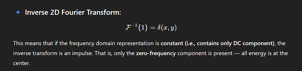
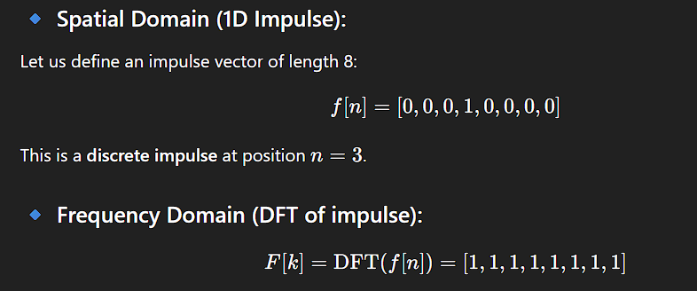
• A single impulse in space ⟷ a constant signal in frequency

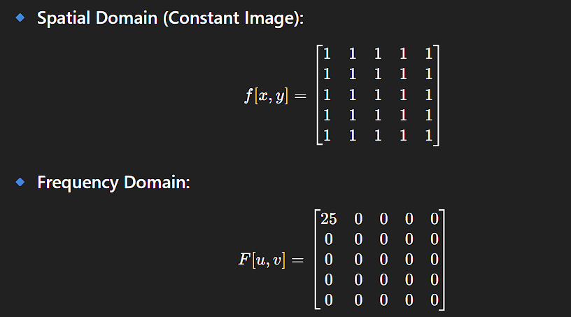
• A constant signal in space ⟷ a single impulse in frequency

---

Frequency Representation of Images

Any function (including an image) that satisfies certain mild conditions can be expressed as a sum of sinusoids with different frequencies and amplitudes.

• Low-frequency components describe regions with slow intensity changes (e.g., smooth walls).
• High-frequency components correspond to sharp transitions (e.g., edges).

Thus, modifying these frequency components changes the appearance of the image:

• Reducing high-frequency components leads to blurring.
• Enhancing high frequencies increases sharpness.

---

Linear Filtering in Frequency Domain

In the spatial domain, linear filtering is done via convolution.

In the frequency domain, it is done via multiplication with a transfer function.

---

Example: 1-D Frequency Domain Filtering

Suppose we want to remove all frequency components above a cutoff u₀ in a 1-D function (like an intensity scan line). This is achieved using a lowpass filter.

• The filter passes frequencies below u₀ and eliminates those above it.
• The corresponding frequency-domain function is called a filter transfer function.

Ideal Lowpass Filter

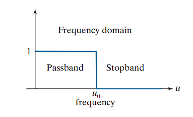
An ideal lowpass filter has an instantaneous transition between passed and blocked frequencies.

• While not physically realizable, it is valuable for theoretical analysis.
• It causes ringing artifacts when implemented digitally.

---

Filtering Procedure in Frequency Domain

1. Compute the Fourier transform of the signal.
2. Multiply the result by the filter transfer function to suppress frequencies above u₀.
3. Take the inverse Fourier transform of the result.
4. The outcome is a blurred version of the original signal.

---

Spatial Domain Equivalent

Due to the spatial-frequency duality:

• The same effect can be achieved by convolution in the spatial domain.
• The equivalent spatial filter kernel is the inverse Fourier transform of the frequency-domain transfer function.

Example:

• If the filter transfer function is a rectangular function (ideal lowpass),
• Then the corresponding spatial filter kernel will show ringing.

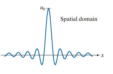
Here the kernel exhibits oscillations due to the abrupt frequency cutoff.

---

Approaches to Constructing Spatial Filters

There are three fundamental approaches for constructing spatial filters in image processing:

---

🔹 1. Mathematical Property-Based Filters

This approach relies on mathematical operations to define filter behavior:

• Averaging filters compute the mean of neighboring pixel values.
  → These tend to blur the image.
  → Mathematically, this is analogous to integration over the neighborhood.

• Derivative filters compute local gradients (changes in intensity).
  → These tend to sharpen the image.
  → Mathematically, this is analogous to differentiation.

This method provides a direct connection between filter behavior and basic mathematical operations.

---

🔹 2. Sampling from 2D Spatial Functions

In this approach, a 2D spatial function is selected for its desirable characteristics, and a spatial filter is constructed by sampling from it.

• Example: Sampling from a Gaussian function to create a weighted-average (lowpass) filter.

• Some of these spatial functions are derived from the inverse Fourier transform of frequency-domain filters.

This method allows for building filters with known shape profiles, such as smooth, symmetric, or isotropic characteristics.

---

🔹 3. Frequency Response-Based Filter Design

This approach begins by specifying a desired frequency response, then designs a spatial filter to approximate that response.

• Typically done through digital filter design techniques.

• A 1D filter with the target frequency response is designed (often with software tools).

• The 1D filter values are then:

  • Expressed as a vector v, and a 2D separable kernel is obtained using:

    w = v · vᵀ

  • Or, rotated about its center to form a circularly symmetric 2D kernel.

This method ensures that the spatial filter adheres closely to frequency-domain specifications, providing precise control over how different frequencies are attenuated or preserved.

---

Smoothing (Lowpass) Spatial Filters

Smoothing, also known as averaging, is a fundamental operation in image processing used to reduce sharp transitions in intensity. Since random noise typically manifests as high-frequency intensity fluctuations, smoothing is a natural tool for noise reduction.

Other applications include:

• Pre-processing before image resampling (to reduce aliasing),
• Reducing irrelevant detail, where “irrelevant” refers to structures smaller than the filter kernel,
• Smoothing false contours caused by insufficient intensity levels,
• Enhancing images when used with techniques like histogram equalization and unsharp masking.

Lowpass filtering refers to applying a filter that removes high-frequency content such as edges, textures, and fine details, while preserving low-frequency variations like gradual illumination changes or shading.

---

🔹 Linear Smoothing Filters

Linear spatial filtering involves convolution of the image with a filter kernel. For smoothing, this convolution process effectively blurs the image. The degree of blurring is controlled by:

• The size of the kernel
• The values of its coefficients

Lowpass filters are foundational, as many other types—such as highpass (sharpening), bandpass, and bandreject filters—are often derived from lowpass filters.

---

Box Filter Kernels

The box filter is the simplest form of lowpass, separable kernel. Its coefficients all have equal values (typically 1), forming a flat-top surface when visualized in 3D—hence the name “box.”

• A general m × n box filter consists of an array of 1s:

  Box Filter = (1 / (m·n)) × [matrix of all 1s]

• The normalization constant is:

  1 / (m·n)

  This ensures:

  1. The output value over a constant region remains equal to that region’s intensity.
  2. The filter does not introduce bias—the total sum of pixel values in the image remains unchanged after filtering.

• Since all rows and columns are identical, the rank of a box kernel is 1, making it separable.

---

🧪 Example : Lowpass Filtering with Box Kernels

A test image of size 1024 × 1024 pixels was filtered using box kernels of size:

• m = 3
• m = 11
• m = 21

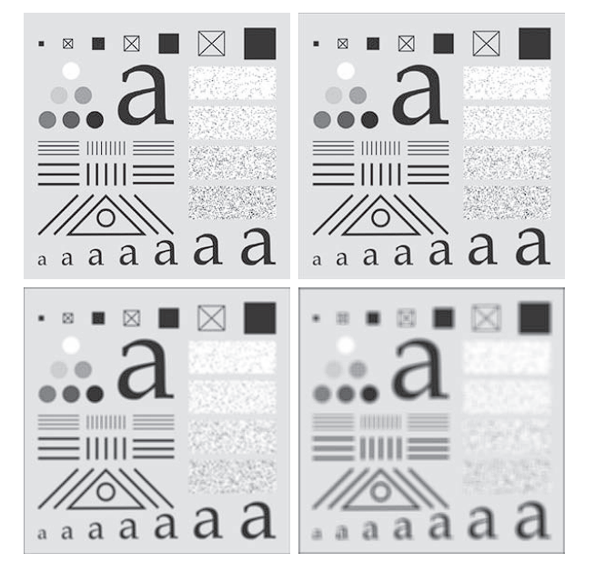
Observations:

• For m = 3:

  • Slight overall blurring.
  • Fine image details (e.g., thin lines and noise) were noticeably affected.
  • A thin gray border appeared due to zero-padding at the boundaries.

• For m = 11:

  • Increased blurring across the image.
  • The dark border due to padding became more pronounced.

• For m = 21:

  • Significant loss of detail across all image components.
  • Smaller structures, such as the small square at the top-left and a character at the bottom-left, lost their shape.
  • The padding artifact expanded, creating a visibly thicker dark border.

---

Note on Zero Padding

Zero padding extends image boundaries by adding rows and columns of zero (black) pixels. While it enables convolution at the edges, it also introduces artifacts, such as dark borders. These are particularly visible when averaging includes zero-valued pixels near the image boundary.

Alternative padding strategies can help eliminate such border artifacts.

---

Limitations of Box Filters

Due to their computational simplicity, box filters are well-suited for rapid prototyping and quick experimentation. In many cases, they produce visually acceptable smoothing results, particularly when minimal processing time is desired. They are also beneficial when the goal is to reduce the impact of smoothing on image edges.

However, box filters exhibit several important limitations that make them unsuitable for precision or perceptually accurate applications.

---

🔹 Limitation 1: Poor Approximation of Lens Blur

In imaging systems, a defocused lens behaves as a lowpass filter. However, box filters fail to replicate the blurring characteristics observed in such optical scenarios.

A single point of light can be modeled by a digital image consisting of all 0s, with a single 1 located at the position of the light point.
When viewed through a defocused lens, this point appears as a fuzzy blob, the size of which increases with the degree of defocus.

Although it might seem intuitive to model this blur using a box kernel, such a filter performs poorly in replicating the smooth, radial falloff of light characteristic of real optical blur.

A Gaussian kernel is a better approximation because its structure mimics the circular symmetry and smooth decay of a defocused point source.

Thus:

• Box filters: Provide uniform weighting and sharp edges → unnatural, blocky blur
• Gaussian filters: Provide smooth, radially symmetric weighting → natural, lens-like blur

---

🔹 Limitation 2: Directional Bias

Box filters inherently favor blurring along perpendicular directions—horizontal and vertical—due to their rectangular, separable structure.

This directional preference can lead to anisotropic blurring, which is problematic in applications involving:

• High-detail imagery
• Strong geometric features (e.g., architectural images, technical drawings)

In such cases, the filter may:

• Produce unnatural smoothing patterns
• Degrade key visual elements (e.g., lines, edges, and corners)

The axis-aligned nature of the box kernel produces non-uniform smoothing artifacts.

---

Circularly Symmetric (Isotropic) Kernels: Gaussian Filters

In many image processing applications where isotropy (orientation independence) is desired, the preferred kernels are circularly symmetric (also called isotropic). This means that the filter response depends only on the distance from the kernel center, not on direction.

Gaussian Kernels

Gaussian kernels of the form

$$w(s,t)=G(s,t)=K{e}^{-\frac{s^2+t^2}{2{\sigma }^2}}$$

are uniquely notable because they are the only circularly symmetric kernels that are also separable

• Here, ( s ) and ( t ) represent spatial coordinates (typically discrete integers for digital images).
• ( K ) is a normalizing constant.
• {sigma} controls the spread (standard deviation) of the Gaussian.

Because Gaussian kernels are separable, they share the computational efficiency advantages of box filters, yet exhibit many additional properties that make them especially well-suited for image processing tasks. These properties will be detailed in the following sections.

The 2D Gaussian kernel $G(x,y)$ can be decomposed into the outer product of two 1D kernels:

$$G(x,y)=G_1(x)\cdot G_2(y)$$

And because the Gaussian function is circularly symmetric, it follows that:

$$G_1=G_2$$

Radial Form of the Gaussian Kernel

By defining the radial distance from the center as

$$r=\sqrt{s^2+t^2}$$

we can rewrite the Gaussian function as a function of ( r ) alone:

$$G(r)=K{e}^{-\frac{r^2}{2{\sigma }^2}}$$

This form emphasizes the circular symmetry of the Gaussian function: its value depends solely on the distance ( r ) from the kernel center, regardless of direction.

---

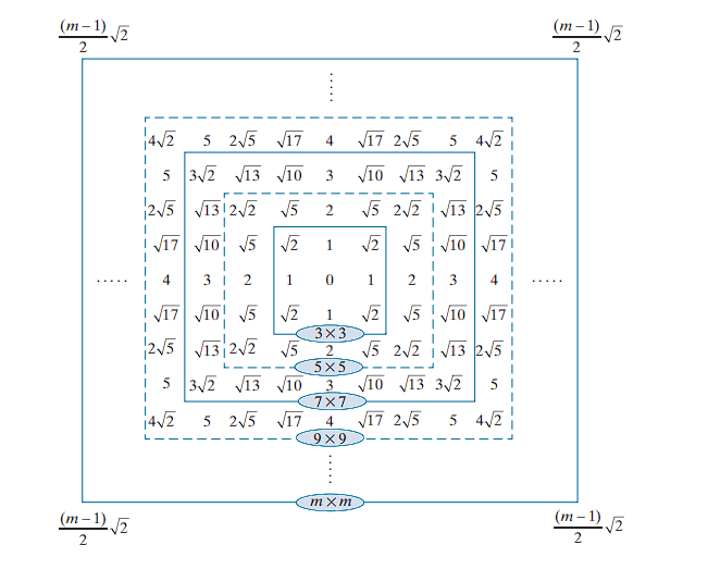
Kernel Size and Distance Calculation

For typical odd-sized kernels (e.g., $m\times m$), the kernel center lies at an integer coordinate, and the squared distance values $r^2$ at each kernel position are also integers.

Specifically, the squared distance to a corner point of the kernel is given by:

$$r_{\text{max}}^2={\left(\frac{m-1}{2}\right)}^2+{\left(\frac{m-1}{2}\right)}^2=2{\left(\frac{m-1}{2}\right)}^2$$

This relation helps in defining the extent of the kernel and in normalizing the Gaussian weights.

---

Kernel Construction by Sampling

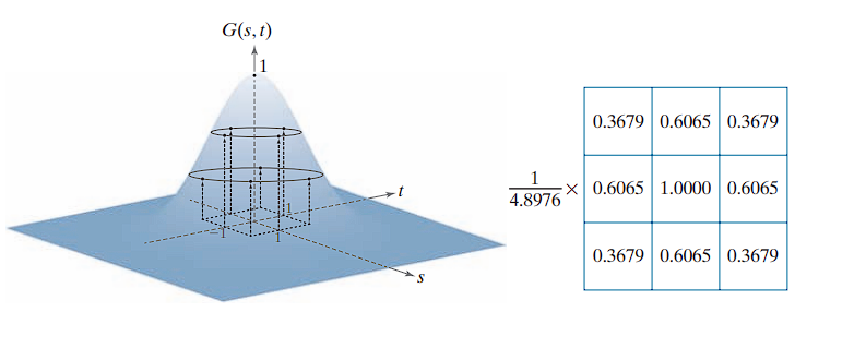
The Gaussian kernel shown above was obtained by sampling with parameters $K=1$ and $\sigma =1$. The process involves:

1. Specifying discrete values of $s$ and $t$ corresponding to kernel coordinates.
2. Evaluating the Gaussian function at each coordinate to obtain kernel coefficients.
3. Normalizing the kernel by dividing each coefficient by the sum of all coefficients, ensuring that the filter preserves the average intensity of uniform regions (similar to box kernel normalization).

---

Separable Implementation

Because Gaussian kernels are separable, the 2-D kernel can be constructed efficiently by:

• Taking samples along a 1-D cross-section through the kernel center to form a vector $\mathbf{v}$.
• Using this vector to generate the 2-D kernel via:

$$\mathbf{K}=\mathbf{v}{\mathbf{v}}^T$$

This separability significantly reduces computational complexity, making Gaussian filtering practical for many real-time and high-resolution image processing tasks.

Separability is one of the many fundamental properties of circularly symmetric Gaussian kernels.

The Gaussian function falls off exponentially.

For example, we know that the values of a Gaussian function at a distance greater than $3\sigma$ from the mean are sufficiently small to be ignored.

$$G(x)=e^{-\frac{x^2}{2{\sigma }^2}}$$

When $(x=3\sigma )$, we substitute into the equation:

$$G(3\sigma )=e^{-\frac{(3\sigma {)}^2}{2{\sigma }^2}}=e^{-\frac{9{\sigma }^2}{2{\sigma }^2}}=e^{-\frac{9}{2}}\approx 0.011$$

Thus, at a distance of $(3\sigma )$ from the center, the Gaussian function has a value of approximately 0.011.

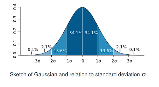
To ensure the kernel includes all significant Gaussian weights,
set the kernel size to cover the range $[-3\sigma ,3\sigma ]$.

Hence, the required minimum size is:

$\text{Size}=2\cdot \lceil 3\sigma \rceil +1$

This implies that if we select the size of a Gaussian kernel to be $L_M\times L_M$, where:

$$L_M=\lceil 6\sigma \rceil$$

(the notation $\lceil c\rceil$ denotes the ceiling of $c$, i.e., the smallest integer not less than $c$), then we are assured of obtaining essentially the same result as if we had used an arbitrarily large Gaussian kernel.

Viewed differently, this tells us that there is no practical benefit to using a Gaussian kernel larger than $L_M\times L_M$ for image processing purposes.

Since we typically use kernels with odd dimensions, we would choose the smallest odd integer that satisfies this condition. For example, if $\sigma =7$, then:

$$L_M=\lceil 6\cdot 7\rceil =\lceil 42\rceil =43$$

So, we would use a $43\times 43$ kernel.

---

Gaussian Convolution: Mean and Standard Deviation

Let $g(x)$ and $h(x)$ be two 1D Gaussian functions with respective means ${\mu }_g$, ${\mu }_h$ and standard deviations ${\sigma }_g$, ${\sigma }_h$. When convolved, the resulting Gaussian $f(x)=g(x)\ast h(x)$ has the following properties:

• Mean of the result:

$${\mu }_{g\ast h}={\mu }_g+{\mu }_h$$

• Standard deviation of the result:

$${\sigma }_{g\ast h}=\sqrt{{\sigma }_g^2+{\sigma }_h^2}$$

This behavior is fundamental in signal and image processing:

• Convolution of two Gaussians yields another Gaussian, centered at the sum of the means and with widened spread due to the combined variances.
• The variances (i.e., ${\sigma }^2$) add under convolution.

This property also underpins the multi-scale nature of Gaussian filtering: repeated applications of Gaussian filters of standard deviations ${\sigma }_1,{\sigma }_2,\dots$ can be combined into a single Gaussian of standard deviation:

$${\sigma }_{\text{total}}=\sqrt{{\sigma }_1^2+{\sigma }_2^2+\dots }$$

So, you can use a single Gaussian filter with ${\sigma }_{\text{total}}$ for the same result.

---

Comparison of Gaussian and Box Kernel Filtering

🔹 Smoothing Characteristics

Gaussian kernels generally need to be larger than box filters to achieve the same degree of blurring. This is due to a key structural difference:

• A box filter assigns equal weight to all pixels within the kernel.
• A Gaussian filter assigns weights that decay with distance from the kernel center, giving less importance to peripheral pixels.

---

🔹 Kernel Size Selection

• There is no significant advantage to using Gaussian kernels larger than $\lceil 6\sigma \rceil \times \lceil 6\sigma \rceil$.

Since kernel sizes must typically be odd integers (for symmetry about the center), we choose the nearest odd integer to $6\sigma$.

For example:

• A $21\times 21$ Gaussian kernel requires approximately $\sigma =3.5$.

• Applying this kernel to the test pattern yields less blurring than a $21\times 21$ box filter To achieve a comparable blurring effect, we need a larger $\sigma$, specifically:

• $\sigma =7$ ⇒ Gaussian kernel size = $43\times 43$

---

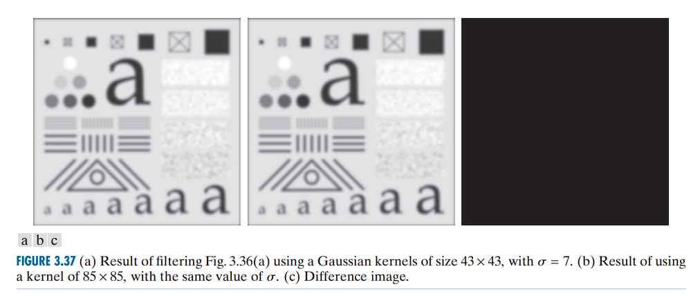
🔹 Effect of Oversized Gaussian Kernels

A larger-than-necessary Gaussian kernels do not provide meaningful improvements in smoothing.

• A $43\times 43$ kernel (minimum size satisfying $6\sigma$, with $\sigma =7$)
• A $85\times 85$ kernel, which is double the size, using the same $\sigma =7$

Observations:

• The result from the $85\times 85$ kernel is visually indistinguishable from that of the $43\times 43$ kernel
• The difference image confirms that the two filtered images differ only slightly, with a maximum pixel difference of 0.75.
• This value is less than one intensity level out of 256 in an 8-bit image, hence negligible in practice.

---

🔹 Comparison of the smoothing effects (Box vs Gaussian)

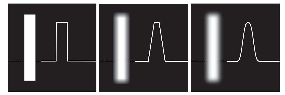
• The box filter produces linear smoothing, characterized by a transition from black to white at the edge that forms a ramp-shaped profile.

  • Key features of the box filter’s edge transition include sharp changes at the beginning and end of the ramp.

  • Such behavior is desirable when preserving sharper edges with less smoothing is important.

• The Gaussian filter, on the other hand, produces significantly smoother edge transitions.

  • The intensity profile transitions more gradually and smoothly around edges.

  • This type of filter is preferable when a generally uniform smoothing effect across the image is required.

• The choice between these filters depends on whether one prefers edge preservation (box filter) or uniform smoothing (Gaussian filter).

---

The effectiveness of a smoothing kernel is not only determined by its size and type, but also by the dimensions of the image being processed. The relative amount of blurring produced by a given smoothing kernel depends directly on the image size.

To achieve comparable blurring on the enlarged image (4096 × 4096), the size and standard deviation of the Gaussian kernel must be scaled proportionally to the image dimensions.

Let:

4096 × 4096 pixels — a fourfold increase in each spatial dimension compared to the original 1024 × 1024 image.

• Original standard deviation: $\sigma =31$
• Scaling factor: 4
• New standard deviation: $\sigma =4\times 31=124$

Thus, the appropriate kernel for the enlarged image should have:

• Size: Closest odd integer to $6\sigma =6\times 124=744$, which is 745 × 745
• Standard deviation: $\sigma =124$
• Normalization constant: $K=1$

Failure to adjust kernel size accordingly can lead to ineffective smoothing or unintended filtering results. This consideration is critical when applying spatial filtering algorithms to images of varying resolution or content scale.

---

Image Padding Techniques and Their Effects on Filtering

zero padding an image introduces dark borders in the filtered output. The thickness and visibility of these borders are determined by both the size and type of the filter kernel applied.

---

🔹 Padding Methods in Image Processing

When performing spatial filtering (such as convolution or correlation), padding becomes necessary to handle the edges of the image where the kernel would otherwise extend beyond the image boundaries. Three common padding methods include:

1. Zero Padding

• Pixels outside the image boundary are assumed to be zero.
• This approach introduces artificial black pixels, leading to dark borders around the filtered image.
• The border’s thickness increases with larger kernel sizes.

2. Mirror (Symmetric) Padding

• Pixels outside the boundary are filled by mirror-reflecting the image across its border.
• This method preserves edge continuity and is most suitable when there are image details near the borders.
• For example, if pixel values near the edge vary significantly, mirror padding avoids sharp discontinuities introduced by zero padding.

3. Replicate Padding

• The values outside the image are set equal to the nearest border value of the image.
• Effective when the image border regions are approximately constant in intensity.
• Maintains a flat extension of the image into the padded region.

---

Use replicate padding if the border areas are uniform.

Use mirror padding if the border contains image features or gradients.

---

Applications of lowpass filtering

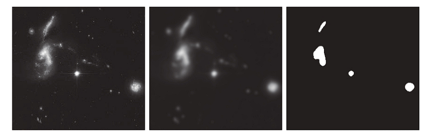
Region Extraction Using Lowpass Filtering

The use of lowpass filtering followed by intensity thresholding to eliminate fine details and extract dominant regions. In this context, irrelevant refers to regions significantly smaller than the filter kernel size.

Procedure

• The image was filtered using a Gaussian kernel of size 151 × 151 (approximately 6% of the image width) with a standard deviation of $\sigma =25$. These parameters were chosen to generate a sharper, more selective Gaussian kernel compared to earlier examples.
• The filtered output highlights four major bright regions while suppressing small-scale details.
• The result of thresholding the filtered image using a threshold value $T=0.4$. Only regions with intensities above the threshold were retained.

This approach effectively isolates the bright regions of interest and suppresses noise or fine structures irrelevant to the application.

Shading Correction Using Lowpass Filtering

Real-world images are often affected by non-uniform lighting or sensor inhomogeneities, which appear as shading or gradual illumination differences across the image. Image shading arises primarily from nonuniform illumination and can adversely affect:

• Quantitative measurements
• Performance of image analysis algorithms
• Human interpretability

Shading correction (also known as flat-field correction) mitigates this by compensating for lighting nonuniformity.

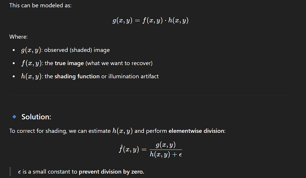
Lowpass filtering is a robust and simple technique for estimating shading patterns.

• A 2048 × 2048 pixel checkerboard image with inner squares of size 128 × 128 pixels.
• The result of applying a Gaussian lowpass filter with a kernel size of 512 × 512, standard deviation $σ = 128$ (equal to the square size), and normalization constant $K = 1$.

This kernel size is four times larger than the square size and sufficient to blur the checkerboard pattern. A kernel only three times the square size would not be adequate.

• The corrected image, obtained by dividing (a) by (b). Though not perfectly flat, this correction significantly improves uniformity.

---

Order-Statistic Filters

Order-statistic filters are nonlinear spatial filters whose output is determined by the ordering (ranking) of the pixel intensity values within the filter’s neighborhood. These filters smooth an image by replacing the center pixel with a value derived from the ranked list of neighboring intensities.

Median Filter

The most well-known order-statistic filter is the median filter. As its name suggests, it replaces the center pixel value with the median of the intensity values within the filter window. This includes the center pixel itself.

Median filtering is especially effective for reducing impulse noise (also known as salt-and-pepper noise), where the noise appears as randomly occurring white and black dots. Compared to linear smoothing filters of similar size, the median filter provides superior noise reduction with significantly less blurring.

Definition

The median, $j$, of a set of $n$ values is the value such that:

• Half the values are $\le j$
• Half the values are $\ge j$

To apply median filtering:

1. Gather all pixel values in the $m\times m$ neighborhood.
2. Sort the values in non-decreasing order.
3. Choose the middle value.

For example:

• In a 3 × 3 window, the median is the 5th largest value.
• In a 5 × 5 window, the median is the 13th largest value.

If duplicate values exist, they are treated normally during sorting.

Example:

suppose a $3\times 3$ neighborhood contains:

(10, 20, 20, 20, 15, 20, 20, 25, 100)

Sorting gives:

(10, 15, 20, 20, 20, 20, 20, 25, 100)

The median is 20.

Thus, the principal function of median filters is to force points to be more like their neighbors. Isolated clusters of pixels that are light or dark with respect to their neighbors—and whose area is less than $m^2/2$ (i.e., one-half the filter area)—are forced by an $m\times m$ median filter to adopt the median intensity of the neighborhood.

The median filter is by far the most useful order-statistic filter in image processing, but it is not the only one. The median corresponds to the 50th percentile of a ranked set of numbers, but other percentiles yield different types of filters.

• The 100th percentile results in the max filter, which is useful for finding the brightest points in an image or for eroding dark areas adjacent to light regions.
  The response of a $3\times 3$ max filter is:

  R_k = \max \{z_1, z_2, ..., z_9\}
  

• The 0th percentile filter is the min filter, used for the opposite purpose.

---

Highpass filtering | Image Sharpening

Image blurring could be accomplished in the spatial domain by pixel averaging (smoothing) within a neighborhood. Because averaging is analogous to integration, it is logical to conclude that sharpening can be accomplished by spatial differentiation.

The strength of the response of a derivative operator is proportional to the magnitude of the intensity discontinuity at the point where the operator is applied. Thus, image differentiation enhances edges and other discontinuities (such as noise) and de-emphasizes areas with slowly varying intensities.

Smoothing is often referred to as lowpass filtering, a term borrowed from frequency domain processing. Similarly, sharpening is often referred to as highpass filtering, where high frequencies responsible for fine details are passed, while low frequencies are attenuated or rejected.

---

Definition of Filter Masks

In image processing, derivative approximations are implemented using discrete filter masks. These masks correspond to finite difference formulas, centered at a specific point x. We assume h = 1 for simplicity.

---

1. Forward Difference Approximation

This estimates the first derivative using the point ahead:

$\frac{f(x+h)-f(x)}{h}$

h = 1

$f(x+1)-f(x)=(-1)\cdot f(x)+(1)\cdot f(x+1)$

This is equivalent to convolving the image with the following kernel / Filter mask: [-1 1]

In 2D (x-direction): We require a 3-element kernel where:

• The center corresponds to f(x, y)
• The right corresponds to f(x+1, y)
• The left corresponds to f(x-1, y) — but is unused in this case, so its coefficient is 0

This gives the following kernel: [0 -1 1]

This is the discrete implementation of the forward derivative.

2. Backward Difference Approximation

This estimates the derivative using the point behind:

$\frac{f(x)-f(x-h)}{h}$

Filter mask: [-1 1 0]

3. Central Difference Approximation

This averages the forward and backward differences:

$\frac{f(x+h)-f(x-h)}{2h}$

Filter mask: : [-1/2, 0, 1/2] = [-1 0 1]

These masks operate by convolving over the image to compute derivatives.

All the above derivative approximations correspond to linear filters, meaning they satisfy:

• Additivity: D(f + g) = D(f) + D(g)
• Homogeneity: D(c · f) = c · D(f)

---

We analyze sharpening filters based on first-order and second-order derivatives.

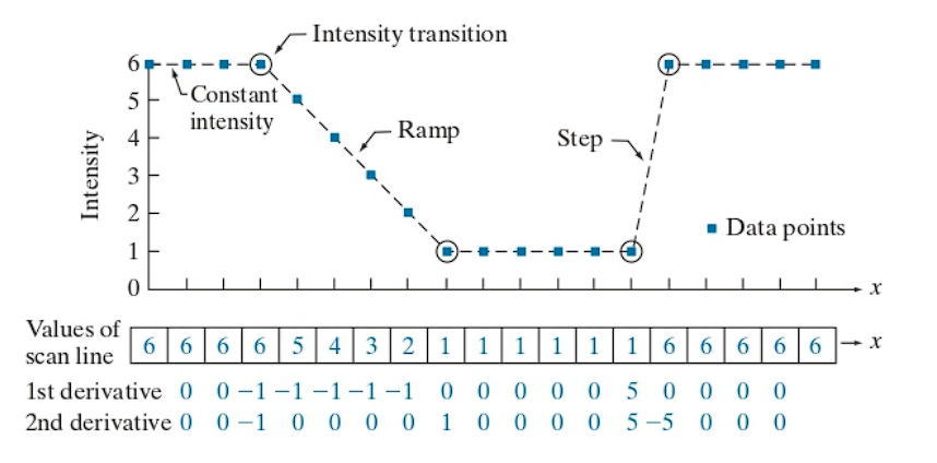
Digital derivatives are defined using differences between pixel values. Definitions must satisfy certain fundamental conditions:

For a First-Order Derivative:

1. Must be zero in areas of constant intensity.
2. Must be nonzero at the onset of a step or ramp.
3. Must be nonzero along intensity ramps.

For a Second-Order Derivative:

1. Must be zero in areas of constant intensity.
2. Must be nonzero at the onset and end of a step or ramp.
3. Must be zero along intensity ramps.

Because pixel values and positions are discrete and finite, the maximum intensity change occurs between adjacent pixels.

A basic definition of the first-order derivative of a one-dimensional function f(x) is the difference:

$\frac{\partial f}{\partial x}=f(x+1)-f(x)$     

We use a partial derivative here to maintain consistent notation when extending to image functions of two variables, f(x, y), where we deal with partial derivatives along the two spatial axes.

The second-order derivative of f(x) is defined as:

$\frac{{\partial }^{2}f}{\partial x^2}=f(x+1)+f(x-1)-2f(x)$     

These definitions satisfy the conditions necessary for discrete differentiation.

In digital images, edges often appear as ramp-like transitions in intensity. In such cases, the first derivative produces thick edges because it remains nonzero along the ramp. Conversely, the second derivative produces a double edge that is one pixel thick, separated by zeros. From this observation, we conclude that the second derivative enhances fine detail more effectively than the first derivative, making it especially suitable for image sharpening (The second derivative clearly identifies both ends of the ramp).It outputs two narrow, sharp pulses, ideal for precise edge detection or sharpening.

Additionally, second derivatives require fewer operations to implement than first derivatives, hence the initial focus on the former.

---

Using the Second Derivative for Image Sharpening — The Laplacian

The method involves defining a discrete approximation of the second-order derivative and constructing a corresponding filter kernel, the objective here is to use isotropic kernels, which yield responses that are invariant to the direction of intensity discontinuities in the image.

It has been demonstrated (Rosenfeld and Kak [1982]) that the simplest isotropic derivative operator for a function f(x, y) is the Laplacian, defined as:

$\frac{{\partial }^{2}f}{\partial x^2}+\frac{{\partial }^{2}f}{\partial y^2}$

Since derivatives of any order are linear operations, the Laplacian is itself a linear operator.

Discrete Formulation

To express the Laplacian in discrete form, we apply the second-order finite difference approximation, now extended to two dimensions.

In the x-direction, we define:

$\frac{{\partial }^{2}f}{\partial x^2}=f(x+1,y)+f(x-1,y)-2f(x,y)$

In the y-direction, we define:

$\frac{{\partial }^{2}f}{\partial y^2}=f(x,y+1)+f(x,y-1)-2f(x,y)$

Adding these two gives the discrete Laplacian of a function f(x, y):

${\nabla }^{2}f(x,y)=f(x+1,y)+f(x-1,y)+f(x,y+1)+f(x,y-1)-4f(x,y)$

Implementation via Convolution

This discrete Laplacian can be implemented using convolution with the following kernel:

0	1	0
1	-4	1
0	1	0

The kernel is isotropic under rotations of 90° with respect to the x- and y-axes. However, this kernel does not account for intensity changes along the diagonal directions. To incorporate these, we expand the discrete Laplacian definition by including four additional terms that capture diagonal intensity differences.

Each diagonal term introduces another -2f(x, y) into the expression, resulting in a modified formulation where the central coefficient becomes -8. The revised kernel, includes contributions from all eight neighboring pixels and is isotropic under 45° rotations as well.

The modified Laplacian kernel is:

1  1  1
1 -8  1
1  1  1

This expanded kernel improves rotational symmetry and yields better isotropic behavior for edge detection and image sharpening across all directions.

Alternate Laplacian Kernels

show two additional commonly used Laplacian kernels. These are derived from negative definitions of the second derivatives compared to those used earlier. Although they produce equivalent results, the sign of the coefficients is inverted, which must be carefully considered when combining a Laplacian-filtered image with the original.

The negative Laplacian kernel corresponding is:

0  -1  0
-1  4  -1
0  -1  0

And the negative isotropic kernel corresponding is:

-1  -1  -1
-1   8  -1
-1  -1  -1

Because the Laplacian is a derivative operator, it emphasizes sharp intensity transitions within an image while de-emphasizing regions of slowly varying intensities. As a result, the output often consists of grayish edge lines and other discontinuities superimposed on a dark, largely featureless background.

To preserve the original image features while maintaining the sharpening effect of the Laplacian, the Laplacian-filtered image is added back to the original image. It is critical to be aware of the sign convention of the Laplacian kernel used:

• If the Laplacian kernel has a negative center coefficient, the sharpened image is obtained by subtracting the Laplacian from the original image.
• If the kernel has a positive center coefficient , the Laplacian is added to the original image.

Formally, the sharpening operation is expressed as:

$g(x,y)=f(x,y)+c\cdot {\nabla }^{2}f(x,y)$

where:

• f(x,y) is the original input image,
• g(x,y) is the sharpened output image,
• ${\nabla }^{2}f(x,y)$ denotes the Laplacian of the image, and
• c is a scalar constant defined as
  • c = -1 if using the kernels is negative center coefficient,
  • c = 1 if using the kernels in positive center coefficient.

This approach ensures proper image sharpening consistent with the sign convention of the discrete Laplacian kernel applied.

The coefficients of each Laplacian kernel sum to zero. Since convolution-based filtering computes a sum of products, when a derivative kernel is applied to a constant region in an image, the convolution result at that location must be zero. This is precisely achieved by using kernels whose coefficients sum to zero.

In contrast, smoothing kernels are normalized so that the sum of their coefficients equals one. This normalization ensures that constant regions in the image remain constant after filtering. Additionally, the sum of pixel values in the original and filtered images remains the same, preventing any bias from being introduced by the smoothing filter.

However, when convolving an image with a kernel whose coefficients sum to zero, the sum of pixel values in the filtered image will also be zero. This implies that the filtered image may contain negative values and often requires additional processing to produce visually suitable results. One such example is adding the filtered image back to the original image.

If an image is filtered with a kernel whose coefficients sum to zero. Then the sum of the pixel values in the filtered image also is zero.

---

First Derivatives and the Gradient in Image Processing

In digital image processing, first-order derivatives are implemented through the magnitude of the gradient of an image.

The gradient of a 2D image function f(x, y) at coordinates (x, y) is defined as the vector:

$\nabla f=\left[\begin{array}{c}\frac{\partial f}{\partial x}\\ \frac{\partial f}{\partial y}\end{array}\right]$

This is a 2D column vector that:

• Points in the direction of the maximum rate of intensity change in the image.
• Is perpendicular to level curves (isointensity contours) of the image at point (x, y).

Gradient Magnitude

The magnitude (or Euclidean norm) of the gradient vector at point (x, y) is given by:

$M(x,y)=|\nabla f|=\sqrt{{\left(\frac{\partial f}{\partial x}\right)}^2+{\left(\frac{\partial f}{\partial y}\right)}^2}$ (Eq. 3-58)

This quantity represents:

• The rate of intensity change at point (x, y) in the direction of the gradient.
• The strength of edges in the image.

By computing the gradient magnitude M(x, y) over all pixel locations, we generate a gradient image, which:

• Has the same dimensions as the original image f(x, y).
• Highlights edges and sharp transitions in intensity.
• Is often referred to simply as the gradient when context is clear.

This gradient image is commonly used in edge detection and image enhancement.

• The components of the gradient vector (∂f/∂x and ∂f/∂y) are linear operators.
• However, the gradient magnitude is nonlinear, due to the squaring and square root operations.
• While partial derivatives are not rotation invariant, the gradient magnitude is (∇f is not rotation invariant while ∣∇f∣ is rotation invariant).
• Edge detection algorithms often use gradient magnitude. Since edges are defined by intensity changes, not their orientation, rotation invariance ensures that edges are detected equally well regardless of how the object is oriented.

Approximate Gradient Magnitude

To simplify computations, the exact magnitude is often approximated using absolute values:

$M(x,y)\approx |\frac{\partial f}{\partial x}|+|\frac{\partial f}{\partial y}|$ (Eq. 3-59)

• This approximation reduces computational cost.
• Isotropy (invariance under rotation) is generally not preserved, except at multiples of 90°, depending on the kernels used. The most popular kernels used to approximate the gradient are isotropic at multiples of 90°. These results are independent, so nothing of significance is lost in using the latter equation if we choose to do so.

---

Discrete Gradient Approximations and Kernel Formulation

We define gradient approximations over a $3\times 3$ region, with pixel intensities labeled $z_1$ through $z_9$:

z1 z2 z3
z4 z5 z6
z7 z8 z9

Basic First-Order Differences

• Horizontal difference: $g_x=z_8-z_5$
• Vertical difference: $g_y=z_6-z_5$

These are derived from simple forward difference approximations.

Roberts Cross-Gradient Operator

Proposed by Roberts (1965), this uses cross differences:

(Eq. 3-60)

• $g_x=z_9-z_5$
• $g_y=z_8-z_6$

---

Gradient Magnitude Using Roberts Operator

• Exact magnitude using squared terms:

  $M(x,y)=\sqrt{(z_9-z_5{)}^2+(z_8-z_6{)}^2}$ (Derived from Eq. 3-58 & 3-60)

• Approximated magnitude using absolute values:

  $M(x,y)\approx |z_9-z_5|+|z_8-z_6|$`

These expressions form the gradient image over the domain of x and y.

---

Implementation with Kernels

The cross differences in Eq. (3-60) are implemented using Roberts cross-gradient kernels:

• For $g_x=z_9-z_5$:

[-1  0]
[ 0  1]

• For $g_y=z_8-z_6$:

[0 -1]
[1  0]

These kernels uses 2×2 kernels and are sensitive to diagonal edges and were historically among the first used for edge detection and is referred to as the Roberts cross-gradient operators.

Sobel Operator

• Modern and Common
• Uses 3×3 kernels with more smoothing

Sobel Approximation of Partial Derivatives

The partial derivatives g_x and g_y are approximated over a $3\times 3$ neighborhood centered on z_5 as follows:

Horizontal Gradient (∂f/∂x):

$$g_x=(z_7+2z_8+z_9)-(z_1+2z_2+z_3)$$

Vertical Gradient (∂f/∂y):

$$g_y=(z_3+2z_6+z_9)-(z_1+2z_4+z_7)$$

These can be implemented by convolving the image with the Sobel kernels:

• For g_x:

[-1  0  1]
[-2  0  2]
[-1  0  1]

• For $g_y$:

[-1 -2 -1]
[ 0  0  0]
[ 1  2  1]

These kernels compute the differences between the first and third rows or columns, effectively capturing changes in intensity along x and y directions, respectively.

---

Gradient Magnitude Using Sobel Operators

Once g_x and g_y are obtained, we compute the gradient magnitude image as:

Using Square Root (Exact):

$$M(x,y)=\sqrt{g_x^2+g_y^2}$$

Using Absolute Values (Approximate):

$$M(x,y)\approx |g_x|+|g_y|$$

$M(x,y)=\sqrt{[(z_7+2z_8+z_9)-(z_1+2z_2+z_3){]}^2+[(z_3+2z_6+z_9)-(z_1+2z_4+z_7){]}^2}$

This expression indicates that the magnitude of the gradient at (x, y) is the square root of the sum of squares of the Sobel-filtered responses in the x and y directions.

Properties of Sobel Kernels

• The center coefficients have a weight of 2 to emphasize the central row/column, achieving smoothing alongside differentiation.
• The sum of all kernel coefficients is zero, ensuring a zero response in regions of constant intensity, as expected from a derivative operator.
• Convolution with these kernels often produces negative values, requiring further processing for visualization.
• The computations of $g_x$ and $g_y$ are linear and performed via convolution.
• The magnitude calculation M(x, y) is nonlinear due to the use of squaring and square roots (or absolute values in approximations).

The Sobel operator is a widely used method for edge detection, providing both differentiation and smoothing. It yields robust results in practice due to its simplicity and effectiveness in detecting intensity transitions in an image, and is isotropic under rotations of 90°.

---