Lecture 05 - Edge Detection & Image Segmentation

NOISE

Noise is an unavoidable artifact in digital images, arising from various physical, electronic, and procedural sources

Sensor-Induced Noise: Modern imaging sensors (e.g., CCD, CMOS) are inherently imperfect. Electronic interference, thermal fluctuations (especially in low-light conditions), and limitations in sensor design introduce randomness in pixel intensities. For example, increasing the ISO in a camera enhances the sensor’s sensitivity, but also amplifies noise.

Modality-Specific Noise:

• In ultrasound imaging, speckle noise is a prominent artifact caused by the constructive and destructive interference of backscattered sound waves. Unlike random noise, speckle has a granular structure that correlates with the tissue texture and imaging method.

• Magnetic Resonance Imaging (MRI) may suffer from Rician noise, while Poisson noise is common in photon-limited modalities like low-light fluorescence microscopy or X-ray imaging.

Noise is modeled probabilistically (Stochastic), not deterministically. Although the exact value at a given pixel cannot be predicted, its distribution can be described. This enables the development of statistical and machine learning-based denoising techniques, which rely on assumptions about the noise distribution.

Additive Noise

Grey values and noise are assumed to be independent. It means that the amount of noise added to a pixel does not depend on the pixel’s original brightness. A dark pixel (e.g., value 10) and a bright pixel (e.g., value 200) are equally likely to have the same amount of noise added to them.

Additive Gaussian Noise : assumes a linear superposition of the original signal and a noise component, which is both independent and Gaussian-distributed.

The observed noisy image is modeled as:

$g(x,y)=f(x,y)+\eta (x,y)$

Where:

• $g(x,y)$ is the observed noisy image
• $f(x,y)$ is the true (unknown) image
• $\eta (x,y)$ is the additive noise term

noise $n$ may obey a variety of distributions, most common is Gaussian distribution

The noise term is modeled as:

$\eta (x,y)\sim \mathcal{N}(0,{\sigma }^2)$

This means that the noise at each pixel is independently drawn from a normal distribution with:

• Mean ($\mu$) = 0
• Variance (${\sigma }^2$) known and fixed

Other Common Noise Models

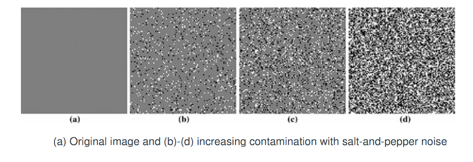
• Salt-and-Pepper Noise: Impulsive in nature; randomly assigns some pixels to minimum or maximum intensity (0 or 255).
  • Salt-and-Pepper Noise is not an additive noise.
  • It doesn’t modify the pixel’s value by adding something. Instead, it replaces random pixels with either the minimum (0) or maximum (255) value
  • 
• Speckle Noise: Multiplicative and structured; often follows Rayleigh or Gamma distributions; common in radar and ultrasound images.
• Poisson Noise: Signal-dependent noise; arises in photon-limited imaging such as low-light photography or microscopy.

Implementing Additive Gaussian Noise in MATLAB

n = random('Normal', 0, 10);  % Generates a single Gaussian noise sample with μ = 0, σ = 10
f = g + n;                    % Adds noise to the original image pixelwise

Measuring the Strength of Additive Gaussian Noise

To evaluate the degradation introduced by Additive Gaussian Noise (AGN) in a noisy image f, compared to the original image g, we use several quantitative metrics.

1. Mean Squared Error (MSE)

The Mean Squared Error is a standard metric that quantifies the average squared difference between the original and noisy images over all pixels.

For an image of size M × N, the MSE is given by:

$\text{MSE}(f,g)=\frac{1}{M\cdot N}{\sum }_{i=1}^M{\sum }_{j=1}^N{\left[f(i,j)-g(i,j)\right]}^2$

• Lower MSE implies that the noisy image is more visually similar to the original.
• It is a direct measure of the noise’s energy relative to the image signal.

---

2. Signal-to-Noise Ratio (SNR)

The Signal-to-Noise Ratio compares the maximum pixel intensity in the image to the noise energy.

$\text{SNR}\_\max =\frac{\max \_x,yf(x,y{)}^2}{\text{MSE}(f,g)}$

• A higher SNR value indicates better visual quality.
• This ratio is unitless and represents relative signal strength.

---

3. Peak Signal-to-Noise Ratio (PSNR)

The Peak Signal-to-Noise Ratio (PSNR) is a logarithmic scale measure, commonly used to evaluate reconstruction quality in image processing.

$\text{PSNR}(f,g)=10\cdot {\log }_{10}\left(\frac{255^2}{\text{MSE}(f,g)}\right)$

• Measured in decibels (dB).
• Assumes 8-bit images (i.e., maximum intensity is 255).
• Higher PSNR values indicate better image quality:
  • ≥ 40 dB: Excellent (imperceptible noise)
  • 30–40 dB: Good
  • 20–30 dB: Acceptable
  • < 20 dB: Poor

Noise is typically hardly visible when PSNR ≥ 30 dB.

---

Image Segmentation

Let R denote the complete spatial domain of an image. Image segmentation is the process of partitioning R into n subregions:

R₁, R₂, ..., Rₙ

These subregions must satisfy the following conditions:

1. Completeness
   Every pixel in the image must belong to a region:

    R = R₁ ∪ R₂ ∪ ... ∪ Rₙ
   

   This ensures that the segmentation fully covers the spatial domain.

2. Connectivity
   Each region Rᵢ must be a connected set:

   Rᵢ is connected, for all i ∈ {1, 2, ..., n}
   

   Connectivity means that every pixel in a region R_i is reachable from any other pixel in R_i by a path that stays entirely within the region.

   A set of pixels is connected if there exists a path (within the region) between any two pixels in that set. This path must obey a selected connectivity rule, commonly one of the following:

   • 4-connectivity: A pixel is connected to its immediate horizontal and vertical neighbors only.
   • 8-connectivity: A pixel is connected to all 8 of its immediate neighbors (including diagonal neighbors).

   The type of connectivity must be predefined.

   Without enforcing connectedness, a region might consist of scattered, unrelated pixels — which is typically not meaningful for segmentation or analysis.

3. Disjointness
   The regions must be mutually exclusive:

    Rᵢ ∩ Rⱼ = ∅, for all i ≠ j
   

4. Homogeneity
   A logical predicate Q(Rᵢ) must be satisfied by all pixels in region Rᵢ:

    Q(Rᵢ) = TRUE, for all i ∈ {1, 2, ..., n}
   

   This predicate defines a property such as intensity uniformity, texture similarity, etc. Each region must satisfy a given property (defined by the predicate Q).

5. Maximality
   For any pair of adjacent regions Rᵢ and Rⱼ, the predicate Q must fail when applied to their union:

    Q(Rᵢ ∪ Rⱼ) = FALSE, if Rᵢ and Rⱼ are adjacent
   

   Two regions are adjacent if their union forms a connected set.

---

Segmentation algorithms for monochrome images generally fall into two basic categories based on intensity properties: discontinuity and similarity.

1. Discontinuity-based Segmentation
   In this category, it is assumed that region boundaries differ significantly from each other and the background, allowing boundary detection by identifying local discontinuities in intensity. Edge-based segmentation is the principal technique employed here.

2. Region-based Segmentation
   Approaches in this category partition an image into regions that are similar according to predefined criteria.

Illustration of discontinuity-based segmentation:

• Figure (a) shows an image composed of a region of constant intensity superimposed on a darker background, also with constant intensity. These two regions constitute the entire image.It has a bright object on a dark background, both uniform regions
• Figure (b) shows the result of detecting the boundary of the inner region based on intensity discontinuities. Pixels inside and outside the boundary are zero (black) because there are no intensity discontinuities there.
• To segment the image, pixels on or inside the boundary are assigned one intensity level (e.g., white), and pixels outside the boundary are assigned another (e.g., black).
• Figure (c) displays the result of this procedure, satisfying segmentation conditions (1) through (3) previously stated.
• The predicate for condition (4) is: If a pixel lies on or inside the boundary, label it white; otherwise, label it black. This predicate holds true for all pixels in Figure (c). Additionally, the two segmented regions (object and background) satisfy condition (5).

illustration of region-based segmentation:

• Figure (d) is similar to Figure (a), except the inner region now exhibits a textured pattern.
• Figure (e) : the result of applying discontinuity-based segmentation. Numerous spurious intensity changes hinder the identification of a unique boundary, making edge-based segmentation unsuitable. Edge-based segmentation struggles because it detects too many false edges, failing to find a unique boundary.
• Alternative approach: However, the outer region remains constant, so a predicate Q, differentiating textured regions from constant regions suffices to solve the segmentation problem.
• The standard deviation of pixel values is a suitable measure here because it is nonzero in textured areas and zero elsewhere.
• Figure (f) illustrates the original image divided into subregions of size 8 × 8. Each subregion was labeled white if the standard deviation of its pixels was positive (predicate TRUE : white if 𝜎>0), and black otherwise.
• If the block has some texture (i.e., variation in intensity),
  → ${\sigma }_k>0$
  → The patch is labeled white (indicating it is part of a textured region).
• If the block is uniform (i.e., all pixel values are the same),
  → ${\sigma }_k=0$
  → The patch is labeled black (indicating it is part of the uniform background).
• This segmentation produces a “blocky” appearance along the region boundary due to uniform labeling of 8 × 8 squares; smaller squares would produce a smoother boundary.
• These results satisfy all five segmentation conditions and works better than edge detection for textured images.

---

Edge-Based Segmentation: Detection of Local Intensity Changes

Segmentation techniques that rely on detecting sharp, localized changes in image intensity - which are signs of important features like:

1. Isolated Points
2. Lines
3. Edges

These features are the foundation of discontinuity-based segmentation, especially edge-based methods.

Edge Pixels and Edge Segments

An edge pixel is defined as a pixel at which the intensity of an image undergoes an abrupt change. A collection of such pixels that are connected forms an edge or edge segment.

Edge detection is typically implemented using edge detectors(Detected using derivatives), which are local image processing operators designed to identify edge pixels.

Lines and Roof Edges

A line in an image can be interpreted as a narrow edge segment in which the intensity of the background on either side of the line differs significantly—either being much higher or much lower—compared to the intensity of the line pixels themselves.

Lines, when analyzed through gradient-based approaches, often produce what are referred to as roof edges due to the gradual transition of intensity values.

Isolated Points

An isolated point may be understood as a foreground pixel entirely surrounded by background pixels, or vice versa. From a processing standpoint, it is a point of high contrast compared to its immediate neighbors, standing out distinctly due to its intensity disparity.

---

Derivatives for Edge Detection in Digital Images

Local averaging smooths an image. Given that averaging is analogous to integration, it is intuitive that abrupt, localized changes in intensity can be effectively detected using derivatives.

To detect sharp changes in intensity (edges), we use derivatives

Specifically, first-order and second-order derivatives are particularly suitable for this task.

Properties of Digital Derivatives

Derivatives of a digital function are defined in terms of finite differences. While there are various methods to compute these differences, approximations for the first and second derivatives must satisfy the following conditions.

• First-order derivative approximations must:

  1. Be zero in regions of constant intensity.
  2. Be nonzero at the onset of an intensity step or ramp.
  3. Be nonzero at points along an intensity ramp.

• Second-order derivative approximations must:

  1. Be zero in regions of constant intensity.
  2. Be nonzero at the onset and end of an intensity step or ramp.
  3. Be zero along intensity ramps.

Given that we are working with digital quantities (i.e., finite values), the maximum possible change in intensity is finite, and the shortest interval over which this change can occur is between adjacent pixels.

---

Taylor Series Expansion

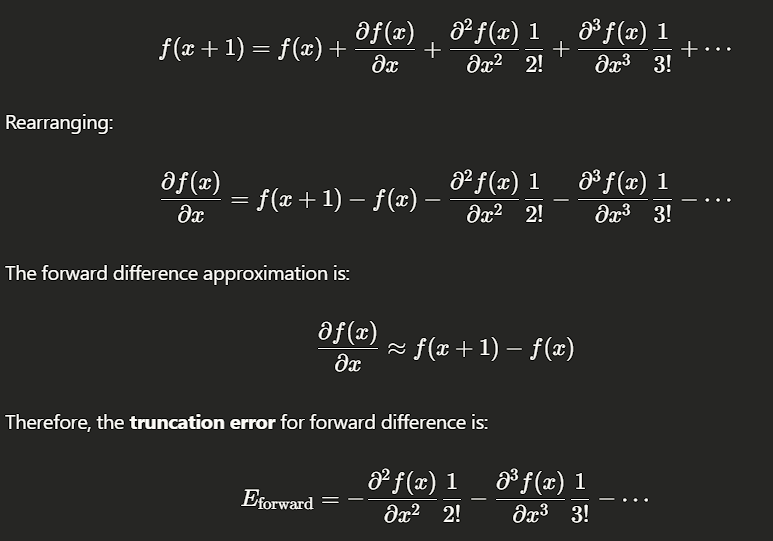
An approximation to the first derivative at an arbitrary point $x$ in a one-dimensional function $f(x)$ can be derived by expanding $f(x+\Delta x)$ into a Taylor series about $x$:

$$f(x+\Delta x)=f(x)+\frac{\partial f(x)}{\partial x}\Delta x+\frac{{\partial }^{2}f(x)}{\partial x^2}\frac{\Delta x^2}{2!}+\frac{{\partial }^{3}f(x)}{\partial x^3}\frac{\Delta x^3}{3!}+\cdots$$

For practical digital processing, the separation $\Delta x$ between samples is measured in pixel units. Conventionally, we let $\Delta x=1$ for the next pixel and $\Delta x=-1$ for the previous pixel.

• When $\Delta x=1$, Equation becomes:

$$f(x+1)=f(x)+\frac{\partial f(x)}{\partial x}+\frac{{\partial }^{2}f(x)}{\partial x^2}\frac{1}{2!}+\frac{{\partial }^{3}f(x)}{\partial x^3}\frac{1}{3!}+\cdots (Eq10-2)$$

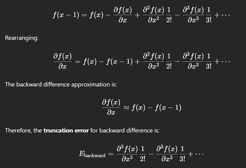
• Similarly, when $\Delta x=-1$:

$$f(x-1)=f(x)-\frac{\partial f(x)}{\partial x}+\frac{{\partial }^{2}f(x)}{\partial x^2}\frac{1}{2!}-\frac{{\partial }^{3}f(x)}{\partial x^3}\frac{1}{3!}+\cdots (Eq10-3)$$

Finite Difference Approximations

By retaining only the linear terms in the series expansions above, we can form approximations to the first derivative using finite differences:

• Forward difference (from Eq. 10-2):

$$\frac{\partial f(x)}{\partial x}\approx f(x+1)-f(x)(Eq10-4)$$

• Backward difference (from Eq. 10-3):

$$\frac{\partial f(x)}{\partial x}\approx f(x)-f(x-1)(Eq10-5)$$

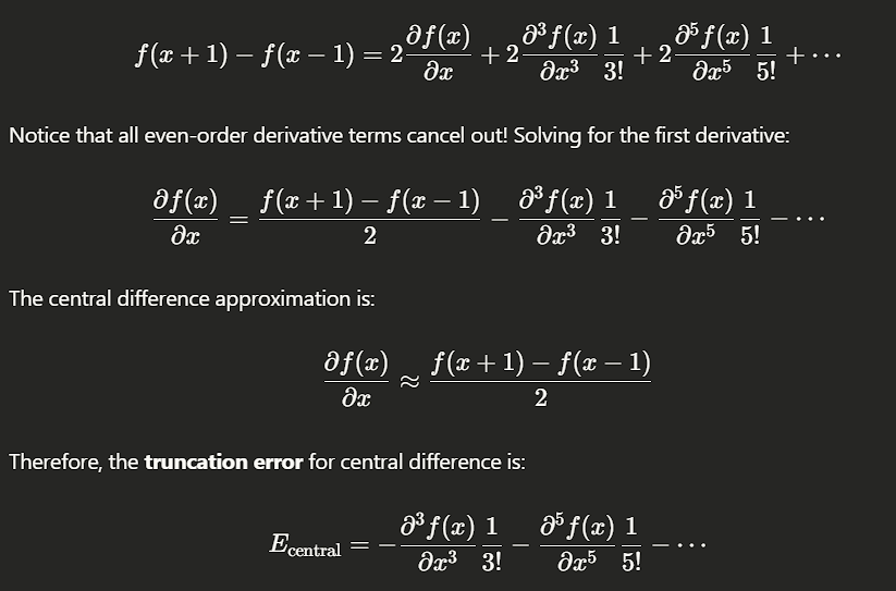
• Central difference (obtained by subtracting Eq. 10-3 from Eq. 10-2):

$$\frac{\partial f(x)}{\partial x}\approx \frac{f(x+1)-f(x-1)}{2}(Eq10-6)$$

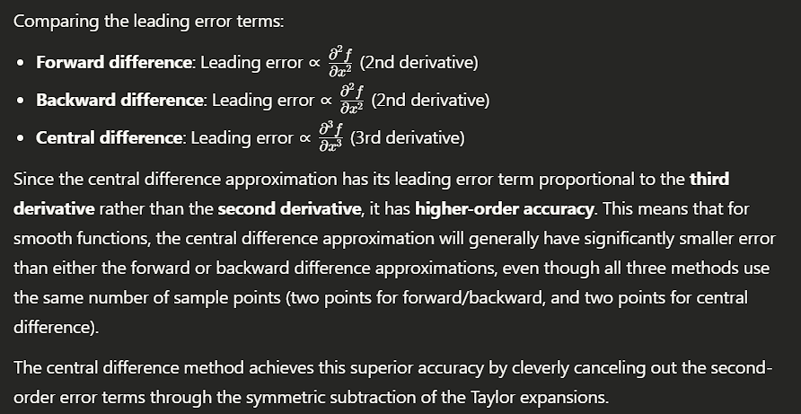
Error Considerations

The higher-order terms that are excluded in the finite difference approximations represent the error between the exact derivative and its approximation. In general, the accuracy of a derivative approximation increases with the number of terms retained from the Taylor series, as this effectively incorporates more neighboring points into the calculation.

However, it has been shown that central difference approximations provide lower approximation error for a given number of points. Consequently, central differences are typically preferred in digital image processing applications when estimating derivatives.

---

Higher-Order Central Derivatives in Digital Image Processing

The second-order derivative based on a central difference, denoted by $\frac{{\partial }^{2}f(x)}{\partial x^2}$, is obtained by adding Equations (10-2) and (10-3). This results in:

$$\frac{{\partial }^{2}f(x)}{\partial x^2}\approx f(x+1)+f(x-1)-2f(x)(Eq10-7)$$

To compute the third-order central derivative, one additional point on each side of $x$ is required. Specifically, we expand $f(x+2)$ and $f(x-2)$ using the Taylor series with $\Delta x=2$ and $\Delta x=-2$, respectively. By combining these expansions and eliminating all derivatives of order less than three, the third-order approximation (ignoring higher-order terms) is given by :

$$\frac{{\partial }^{3}f(x)}{\partial x^3}\approx -f(x+2)+2f(x+1)-2f(x-1)+f(x-2)(Eq10-8)$$

Similarly, the fourth-order finite difference, which is the highest derivative considered in the text, is derived using additional Taylor expansions and eliminating terms up to the third order. The result is:

$$\frac{{\partial }^{4}f(x)}{\partial x^4}\approx f(x+2)-4f(x+1)+6f(x)-4f(x-1)+f(x-2)(Eq10-9)$$

Summary of Central Difference Formulas

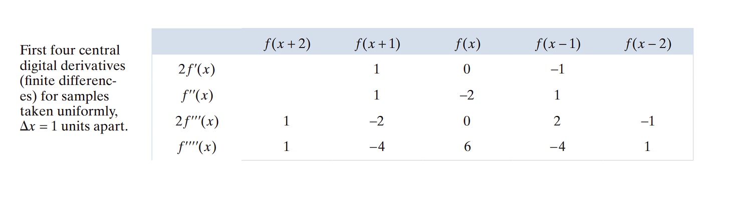
One key observation is the symmetry of the coefficients about the center point x. This symmetry contributes to the lower approximation error of central differences, compared to forward or backward differences, for a given number of points.

Extension to Two Variables

For functions of two variables, the same central difference formulas are applied independently to each variable:

• Second derivative with respect to $x$:

$$\frac{{\partial }^{2}f(x,y)}{\partial x^2}\approx f(x+1,y)+f(x-1,y)-2f(x,y)(Eq10-10)$$

• Second derivative with respect to $y$:

$$\frac{{\partial }^{2}f(x,y)}{\partial y^2}\approx f(x,y+1)+f(x,y-1)-2f(x,y)(Eq10-11)$$

These approximations are consistent with the properties required of first- and second-order derivatives.

Illustration of the behavior of these derivatives:

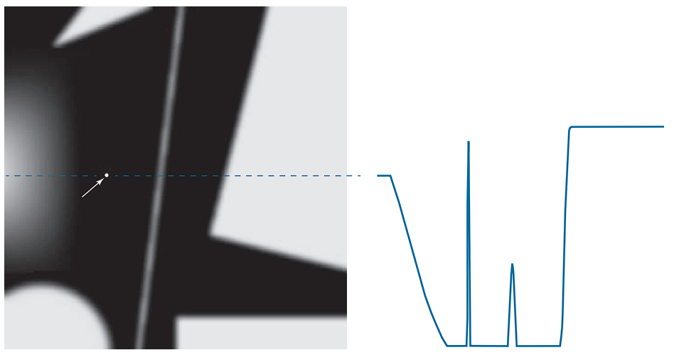
• (a) displays an image containing various objects, a line, and an isolated point.
• (b) presents a horizontal intensity profile (scan line : A horizontal or vertical line or even diagonal that you draw across an image to sample the intensity values of the pixels along that line, and Plot those values as a function of position) through the center of the image, including the isolated point.

The intensity transitions observed along this scan line demonstrate two edge types:

• Ramp edges (gradual transitions) on the left
• Step edges (abrupt transitions) on the right

Additionally, transitions associated with thin objects, such as lines, often manifest as roof edges.

---

Behavior of First- and Second-Order Derivatives

🔷 What is a Ramp Edge?

  A ramp is a gradual change in intensity across multiple pixels.

  It can go from dark to light or light to dark — the direction does not define a ramp; it's the smoothness of the transition.

  The slope is consistent, meaning the brightness increases or decreases steadily

🔷 What is a Step Edge?

  A step edge is a sudden change in intensity between two adjacent pixels.

  There is no gradual slope — the change is abrupt.

  Ex : 20, 20, 100, 100 → Step edge at transition from 20 → 100

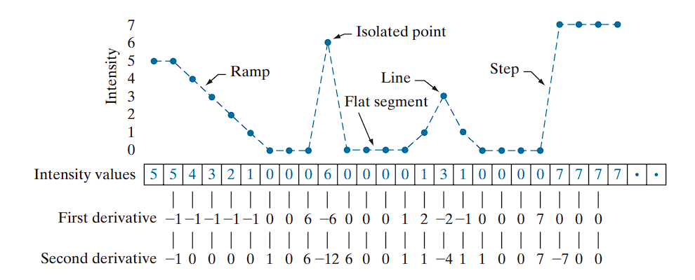
As we traverse this profile from left to right, the following properties are observed:

1. Ramp Edge:

   • The first-order derivative is nonzero at the onset and along the ramp.
   • The second-order derivative is nonzero only at the onset and end of the ramp.
   • This implies that first-order derivatives produce “thick” edges, while second-order derivatives yield thinner edges.

2. Isolated Noise Point:

   • The second-order derivative produces a stronger response than the first-order derivative.
   • This is expected, since second-order derivatives amplify sharp intensity changes more aggressively, including fine details and noise.

3. Thin Line:

   • Again, the second derivative response is stronger, further confirming its sensitivity to such features.
   • This type of pattern produces a roof edge in the intensity profile, characterized by a narrow peak or ridge surrounded by symmetric slopes.
   • The second derivative shows a distinct positive–negative–positive pattern around the peak, creating a double-edge effect that helps localize both sides of the line.

4. Step Edge:

   • For both ramp and step edges, the second-order derivative exhibits opposite signs as it enters and exits the edge region.
   • This “double-edge” effect is crucial in edge detection.
   • Additionally, the sign of the second derivative can be used to determine edge polarity:
     • A negative second derivative indicates a transition from light to dark.
     • A positive second derivative indicates a transition from dark to light.

The Step Edge

Key conclusions:

1. First-order derivatives generally result in thicker edge profiles.
2. Second-order derivatives respond more strongly to fine details, including noise, isolated points, and thin lines.
3. Second-order derivatives produce a double-edge effect at ramp and step intensity transitions.
4. The sign of the second derivative can help determine whether an edge transition is from light to dark or vice versa.

---

Derivatives via Spatial Convolution

To compute first and second derivatives at every pixel location in an image, the standard method is spatial convolution.

For a $3\times 3$ filter kernel, the convolution procedure is as follows:

At each pixel, compute the sum of the products of the kernel coefficients with the intensity values of the pixels in the region covered by the kernel. Mathematically, the response at the center pixel is given by:

$$Z=\sum _{k=1}^9{z}_k{w}_k$$

Where:

• $z_k$ is the intensity value at the $k^{\text{th}}$ pixel under the kernel,
• $w_k$ is the corresponding kernel coefficient.

This convolution-based approach applies to any linear filter used for computing local derivatives across the image.

---

Detection of Isolated Points Using the Laplacian

Point detection should be based on the second-order derivative, which is implemented using the Laplacian operator:

$${\nabla }^{2}f=\frac{{\partial }^{2}f}{\partial x^2}+\frac{{\partial }^{2}f}{\partial y^2}$$

The partial derivatives are computed using the second-order finite differences from Eqs. (10-10) and (10-11). Substituting those into the Laplacian yields:

$${\nabla }^{2}f(x,y)=f(x+1,y)+f(x-1,y)+f(x,y+1)+f(x,y-1)-4f(x,y)\text{ (Eq 10-14)}$$

There are two common versions of the 2D Laplacian operator, based on how many neighbors they use:

---

1. 4-Connected Laplacian (Only vertical and horizontal neighbors)

${\nabla }^{2}f(x,y)=f(x+1,y)+f(x-1,y)+f(x,y+1)+f(x,y-1)-4f(x,y)$

Corresponding kernel:

$$\left[\begin{array}{ccc}0& 1& 0\\ 1& -4& 1\\ 0& 1& 0\end{array}\right]$$

---

2. 8-Connected Laplacian (Includes diagonals too)

${\nabla }^{2}f(x,y)={\sum }_{\text{all 8 neighbors}}f(x+i,y+j)-8f(x,y)$

Corresponding kernel:

$$\left[\begin{array}{ccc}1& 1& 1\\ 1& -8& 1\\ 1& 1& 1\end{array}\right]$$

• The −4 version is simpler and less sensitive to diagonal structures.
• The −8 version gives a stronger and more symmetrical response, especially useful for detecting points and lines in all directions.

---

Point Detection via Thresholding

We consider that a point has been detected at a location ( (x, y) ) if the absolute value of the filter response at that point exceeds a specified non-negative threshold ( T ). The output image is then binary, where detected points are labeled 1, and all others 0:

$$g(x,y)=\{\begin{array}{ll}1& \text{if }|Z(x,y)|>T\\ 0& \text{otherwise}\end{array}$$

Where:

• ( g(x, y) ) is the binary output image,
• ( Z(x, y) ) is the response computed using spatial convolution,
• ( T ) is the threshold.

This procedure measures weighted differences between a pixel and its 8-neighbors. The intuition is that the intensity of an isolated point differs significantly from its neighborhood, making it detectable by this kernel. The kernel coefficients sum to zero, ensuring that areas of constant intensity produce a zero response, as is typical for derivative filters.

---

Example: Detection of Isolated Points in an Image

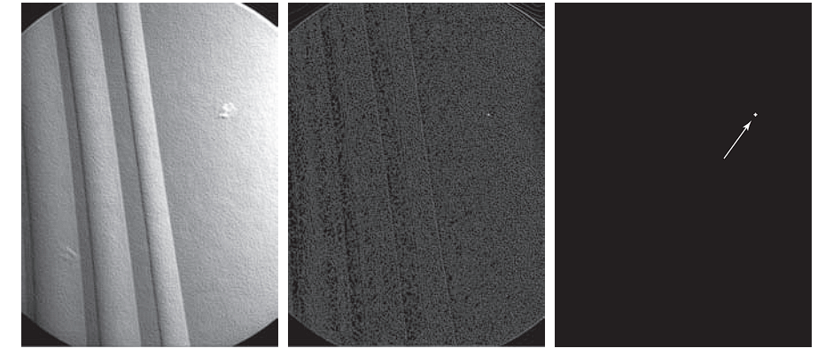
• (a) An X-ray image of a turbine blade from a jet engine.

• The blade exhibits porosity, shown as a single black pixel in the upper-right quadrant.

• (b): Result of filtering the image using the Laplacian kernel.

• (c): Result of thresholding with:

  $T=0.9\cdot \max \left(|Z(x,y)|\right)$

• The isolated pixel is clearly visible at the tip of the arrow (enlarged for visibility).

This method is effective when intensity changes occur abruptly at single-pixel locations, surrounded by a homogeneous background. When this condition is not satisfied, other edge or region detection methods are more appropriate.

---

Line Detection

Second-order derivatives provide a stronger response and yield thinner line representations than first-order derivatives. Therefore, the Laplacian kernel is also applicable for detecting lines. However, care must be taken to manage the double-line effect produced by second derivatives.

---

Using the Laplacian for Line Detection

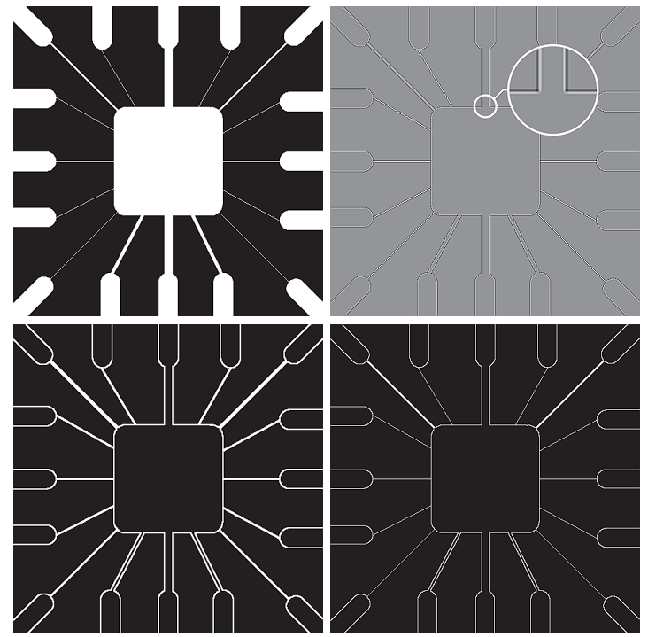
• (a) shows a 486 × 486 binary portion of a wire-bond mask for an electronic circuit.
• (b) presents its Laplacian-transformed image. Since the Laplacian output includes negative values, scaling is necessary for display.
  • In this image:
    • Mid gray denotes zero.
    • Darker shades indicate negative values.
    • Lighter shades indicate positive values.
  • The double-line effect (one light stripe, one dark stripe) is evident in the magnified view of the image.

---

Handling the Laplacian Output

A naive approach might suggest taking the absolute value of the Laplacian image to mitigate the presence of negative values. However:

• (c) : ∣Laplacian(x,y)∣ demonstrates that this approach doubles the line thickness, which is generally undesirable.
• A better approach is to use only the positive values of the Laplacian image.
  • In noisy images, apply a positive threshold to ignore minor fluctuations around zero.
• (d) : if Laplacian(x,y)>T, keep it; else 0
  • This method shows that this selective positive filtering yields thinner and more accurate line detections.

---

Considerations on Line Width and Kernel Size

• Observe that in (b)–(d), wide lines (relative to the kernel size) exhibit a zero “valley” between the edges of the lines.
  • This occurs because when a 3 × 3 kernel is centered on a line of constant intensity and width of 5 pixels, the filter response is zero, creating the observed effect.
  • zero valley —> a flat region the Laplacian ignores because it has no local intensity change.
  • Ex :

So, line detection works best when the kernel can “wrap around” the entire line:

• Assume lines are thin relative to the detector’s kernel.
• If the line is too wide, like 3+ pixels, the center becomes flat — it looks like a region, not an edge.
• Wide lines should instead be considered as regions, and processed using the edge detection techniques

---

Directional Line Detection Using Kernels

The Laplacian detector kernel is isotropic, meaning its response is independent of direction—across vertical, horizontal, and diagonal orientations in a 3 × 3 neighborhood. However, in many applications, the goal is to detect lines oriented in specific directions.

---

Directional Kernels

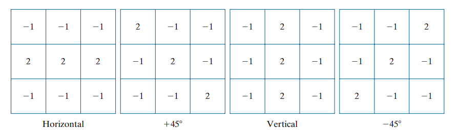
When an image with a constant background and embedded lines oriented at 0°, ±45°, and 90° is filtered with each kernel, the maximum response occurs when a line of interest aligns with the preferred orientation of the kernel:

• The first kernel responds maximally to horizontal lines (0°).
• The second kernel to +45° diagonal lines.
• The third kernel to vertical lines (90°).
• The fourth kernel to −45° diagonal lines.

Each kernel emphasizes its intended direction by weighting the central axis with a coefficient of 2, while maintaining zero sum overall to ensure no response in uniform-intensity regions.

---

Response and Selection

Let the outputs of the four directional kernels be denoted as:
Z₁, Z₂, Z₃, and Z₄ — corresponding to the four kernels. These outputs are computed using the spatial convolution defined as:

$$Z=\sum _{k=1}^9{w}_k\cdot z_k$$

At any point in the image:

• If Zₖ > Zⱼ for all j ≠ k, then that point is most likely part of a line oriented in direction k.

For instance, if at a pixel, Z₁ is the maximum among all four responses (|Z1| > |Zj| for j = 2,3,4), the point is associated with a horizontal line.

---

Thresholding Directional Responses

To extract lines in a specific orientation (e.g., +45°), the following steps are followed:

1. Convolve the image with the corresponding directional kernel.
2. Threshold the positive response:

$$g(x,y)=\{\begin{array}{ll}1,& \text{if }Z(x,y)>T\\ 0,& \text{otherwise}\end{array}$$

where T is a positive threshold value selected based on the maximum observed response.

3. The output is a binary image in which 1 corresponds to points strongly aligned with the kernel direction.

---

Example: Detecting Lines at +45°

We are interested in identifying one-pixel-thick lines oriented at +45°

• Kernel used: Second directional kernel
• (b) shows the filtered result. The darker and lighter regions indicate negative and positive responses, respectively.

There are two significant segments oriented at +45°:

• Top-left corner: Segment is not one pixel thick → yields weaker response.
• Bottom-right corner: Segment is one pixel thick → yields stronger response .

Thresholding the Response

• From (e), we extract positive values of the Laplacian response.
• Select threshold T = 254 (one less than the maximum value).
• (f) shows the binary output using the rule g(x, y) > T, with detected points marked in white.

Some isolated points also exceed the threshold. These result from local configurations that accidentally align with the kernel’s preferred direction.

To address this:

• Use the Laplacian kernel to detect and eliminate such isolated points, or
• Apply morphological operators for cleanup.

---

Edge Models

An edge model describes the shape of intensity change across an edge. It’s a 1D profile — like scanning across an edge and plotting how the pixel intensity changes. Edge detection is a fundamental technique in image segmentation, focused on identifying abrupt (local) intensity changes.

---

Classification of Edge Models by Intensity Profile

Edge models are typically classified by their intensity transition profiles:

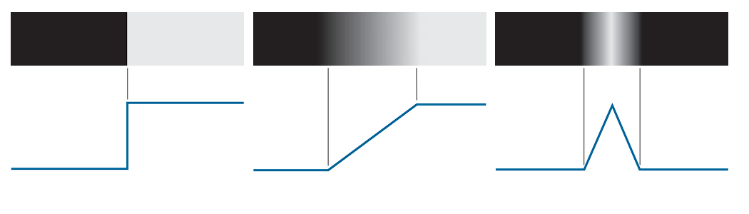
1. Step Edge

A step edge represents an ideal transition between two intensity levels, ideally over one pixel.

• (a) shows a section of a vertical step edge and the corresponding horizontal intensity profile.
• These occur in synthetic images, such as those from solid modeling or animation.
• If no smoothing is applied, the edge remains one-pixel wide.
• Step-edge models are frequently used for algorithm development (e.g., the Canny edge detector was derived using this model).

2. Ramp Edge

In real-world images, due to focus limitations (e.g., lens aberrations) and sensor noise, edges are usually blurred.
These are more accurately modeled as ramp edges, as shown in (b):

• The slope of the ramp is inversely proportional to the degree of blurring.
• There is no single edge point. Instead, any point on the ramp is considered part of the edge.
• An edge segment consists of connected ramp points.

3. Roof Edge

A roof edge models thin line-like features.(c):

• The base width depends on the thickness and sharpness of the line.
• In the limit of a one-pixel-wide base, the roof edge becomes a one-pixel-thick line.
• Examples:
  • Range imaging (e.g., pipes closer to the sensor than the wall).
  • Digitized line drawings.
  • Satellite imagery (e.g., roads modeled as roof edges).

It is common to find all three types of edges in a single image. Although noise and blur alter the profiles, reasonably sharp edges retain a resemblance to these idealized models.

---

Practical Use of Edge Models

The benefit of these models is that they enable the formulation of mathematical representations of edges, which are essential for algorithm development. The performance of an edge detector depends on how closely real image content matches the model used in its derivation.

---

Behavior of Derivatives

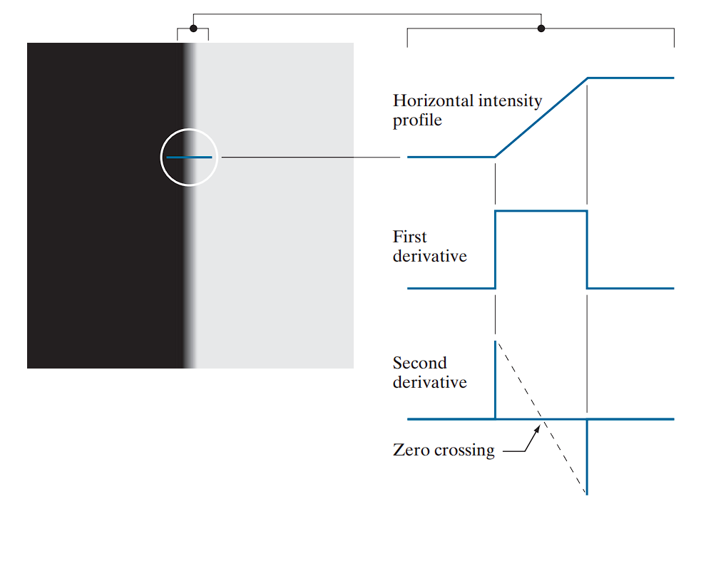
From left to right along the ramp:

• The first derivative:

  • Is positive at the onset of the ramp and on the ramp itself.
  • Is zero in constant-intensity regions.

• The second derivative:

  • Is positive at the beginning of the ramp.
  • Is negative at the end of the ramp.
  • Is zero on the ramp and in constant regions.

If the edge transitions from light to dark, the signs are reversed.

The zero crossing of the second derivative is defined by the intersection of the intensity axis and a line between the extrema of the second derivative. This point is used to localize the center of thick edges.

---

Key Observations

1. The magnitude of the first derivative can be used to detect the presence of an edge.
2. The sign of the second derivative helps identify which side of the edge (light or dark) a pixel lies on.
3. The second derivative:
   • Produces two values per edge (at the start and end of the ramp).
   • Its zero crossings provide accurate localization of the edge center.

---

Generalization to 2D Images

We’ve been looking at how intensity changes along a single row of pixels (like left to right). But real images are 2D — intensity can also change vertically, diagonally, etc. Although the analysis above applies to a 1D horizontal profile, it generalizes naturally:

• At any point on an edge, define a 1D profile perpendicular to the edge orientation.
• Apply the same interpretation of the first and second derivatives.

---

Some models include smooth transitions into and out of the ramp, but the conclusions remain largely consistent with the ideal ramp. Real-world edges aren’t perfect. They often fade in and out gradually (i.e., not ideal ramps), but the same derivative behavior still appears. Using the simplified ramp model facilitates theoretical development without significant loss of generality.

---

Behavior of the First and Second Derivatives in the Region of a Noisy Edge

The edge models shown in above are idealized and free of noise. However, real images often include noise, which affects edge detection significantly. To analyze this, below presents image segments showing four ramp edges transitioning from black (left) to white (right)—representing a single edge transition.

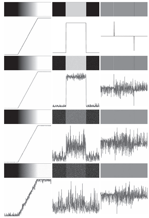
Noise Levels in Edge Images

• The top-left image is free of noise.
• The remaining three images (first column) are corrupted with additive Gaussian noise of:
  • Mean = 0
  • Standard deviations: $\sigma =0.1$, $1.0$, and $10.0$ intensity levels
• All images have 8-bit resolution:
  • Intensity range: $0$ (black) to $255$ (white)
• Below each image is a horizontal intensity profile through the image center.

---

Behavior of the First Derivative

Consider the top of the center column, which shows the first derivative of the noiseless edge:

• In constant regions, the derivative is zero (appearing as black bands).
• On the ramp, the derivative is constant and non-zero, equal to the slope of the ramp (shown in gray).
• As we move down the column, the derivatives deviate significantly due to noise:
  • With increasing noise, it becomes harder to associate the resulting profile with that of a ramp.
  • Notably, even when noise is visually undetectable in the original images, it strongly disrupts the derivatives.

This highlights the sensitivity of the first derivative to noise.

---

Behavior of the Second Derivative

The rightmost column shows the corresponding second derivatives:

• In the noiseless image:

  • Thin white and black vertical lines represent the positive and negative components of the second derivative, respectively.
  • Gray represents zero response

• As noise increases:

  • The second derivative becomes even more sensitive to noise than the first.
  • Only the case with $\sigma =0.1$ slightly resembles the noiseless profile.
  • Because the second derivative involves differences of differences, it amplifies even tiny changes in intensity.
  • The remaining second-derivative images are heavily distorted, making it difficult to detect the positive and negative lobes, which are essential for locating edges via zero crossings.

These results demonstrate that even low levels of visual noise can severely impact the performance of derivative-based edge detectors.

Implication | The Solution:

Image smoothing must be seriously considered before applying derivative operations in edge detection, especially in noisy environments.

---

Typical Steps in Edge Detection

Given the effects of noise and the sensitivity of derivative operations, edge detection typically involves three sequential steps:

1. Image Smoothing (Noise Reduction):

   • Necessary to reduce the impact of noise.

2. Edge Point Detection:

   • A local operation that identifies all pixels that are potential edge-point candidates.

3. Edge Localization:

   • Selects from the candidates only those that form connected edge segments.

---

Basic Edge Detection

Detecting changes in intensity for the purpose of identifying edges can be accomplished using first- or second-order derivatives.

The Image Gradient and Its Properties

The principal tool for determining edge strength and direction at any point $(x,y)$ in an image $f$ is the gradient, denoted by $\nabla f$, and defined as the vector:

$$\nabla f(x,y)\equiv \left[\begin{array}{c}{g}_x(x,y)\\ g_y(x,y)\end{array}\right]=\left[\begin{array}{c}\frac{\partial f(x,y)}{\partial x}\\ \frac{\partial f(x,y)}{\partial y}\end{array}\right]$$

• The gradient vector $\nabla f(x,y)$ points in the direction of the maximum rate of change of $f$ at $(x,y)$.
• When computed for all applicable values of $x$ and $y$, $\nabla f(x,y)$ becomes a vector field (gradient image).

---

Gradient Magnitude

The magnitude $M(x,y)$ of the gradient vector at point $(x,y)$ is given by the Euclidean norm:

$$M(x,y)=|\nabla f(x,y)|=\sqrt{g_x^2(x,y)+g_y^2(x,y)}$$

• $M(x,y)$, $g_x(x,y)$, and $g_y(x,y)$ are arrays of the same size as the image $f(x,y)$.
• Elementwise operations are used throughout (see Section 2.6).

---

Gradient Direction

The direction $\alpha (x,y)$ of the gradient vector is:

$$\alpha (x,y)={\tan }^{-1}\left(\frac{g_y(x,y)}{g_x(x,y)}\right)$$

• Angles are measured counterclockwise from the x-axis
• The edge direction is orthogonal to the gradient direction at the point.

---

Computing the Gradient: An Example

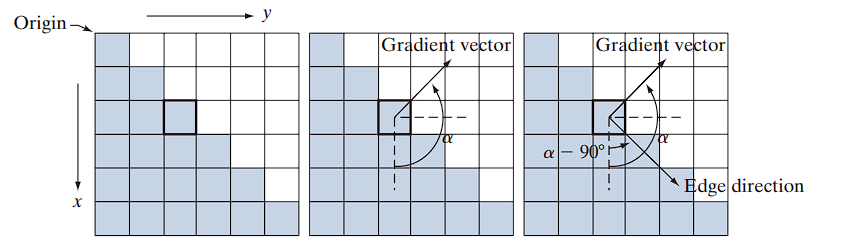
(a) illustrates a zoomed section of an image with a straight edge segment:

• Each square represents a pixel.
• White pixels: intensity value = 1
• Shaded pixels: intensity value = 0
• The highlighted box marks the point of interest.

To compute gradient components:

1. Use a $3\times 3$ neighborhood centered on the point.
2. Approximate partial derivatives:
   • In the $x$-direction: subtract top row values from bottom row values.
   • In the $y$-direction: subtract left column values from right column values.

From this:

• $\frac{\partial f}{\partial x}=-2$
• $\frac{\partial f}{\partial y}=2$

Then,

$$\nabla f=\left[\begin{array}{c}{g}_x\\ g_y\end{array}\right]=\left[\begin{array}{c}-2\\ 2\end{array}\right]\Rightarrow |\nabla f|=\sqrt{(-2{)}^2+2^2}=\sqrt{8}$$

Gradient Direction:

$$\alpha ={\tan }^{-1}\left(\frac{2}{-2}\right)={\tan }^{-1}(-1)=-45^{\circ }$$

In positive counterclockwise direction, this corresponds to:

$$\alpha =135^{\circ }$$

---

Edge Direction

Since the edge direction is orthogonal to the gradient vector:

$${\theta }_{\text{edge}}=\alpha -90^{\circ }=135^{\circ }-90^{\circ }=45^{\circ }$$

• All edge points in (a) share the same gradient.
• The edge segment is therefore aligned in a uniform direction.

---

Terminology

• The gradient vector is also known as the edge normal.
• When normalized to unit length, it is referred to as the edge unit normal.

---

Gradient Operators

Obtaining the gradient of an image requires computing the partial derivatives $\partial f/\partial x$ and $\partial f/\partial y$ at every pixel location in the image. For the gradient, we typically use either forward or centered finite differences. Using forward differences, we obtain:

• $g_x(x,y)=f(x+1,y)-f(x,y)$
• $g_y(x,y)=f(x,y+1)-f(x,y)$

These equations are implemented over the entire image $f(x,y)$ by filtering with the 1-D kernels : .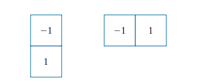

---

Roberts Cross Operators

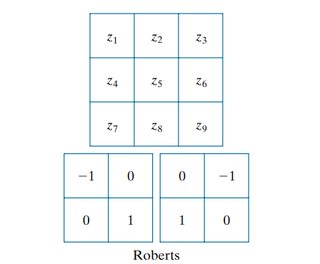
When diagonal edge directions are of interest, 2-D kernels are used. The Roberts cross-gradient operators (Roberts [1965]) represent an early approach to this. Consider the $3 × 3$ region in (a). The Roberts operators are defined by:

• $g_x=z_9-z_5$
• $g_y=z_8-z_6$

These differences are implemented via filtering with the corresponding kernels shown above

Although $2 × 2$ kernels are simple, they are less effective at capturing edge directional information. This limitation arises from their lack of symmetry about the center pixel.

In digital image processing, we often use a different coordinate system:

The origin (0,0) is at the top-left corner,

The x-axis increases rightward,

The y-axis increases downward.

[ G_x = f(x, y) - f(x+1, y+1) ]

This measures the difference between the top-left and bottom-right, the Roberts $G_x$ detects edges along +45°, corresponding to the ↘ direction.

---

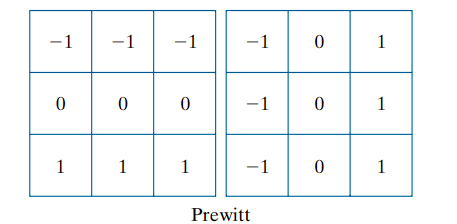
Prewitt Operators

The smallest symmetric kernels suitable for directional edge detection are of size 3 × 3. These consider data on both sides of the center point and thus encode more directional information. The Prewitt operator approximations for partial derivatives are:

• $g_x=(z_7+z_8+z_9)-(z_1+z_2+z_3)$
• $g_y=(z_3+z_6+z_9)-(z_1+z_4+z_7)$

Here, the difference between the third and first rows approximates ∂f/∂x, and the difference between the third and first columns approximates ∂f/∂y. These kernels are implemented using :

---

Sobel Operators

A refinement of the Prewitt operator uses a weight of 2 in the center row/column for added smoothing:

• $g_x=(z_7+2z_8+z_9)-(z_1+2z_2+z_3)$
• $g_y=(z_3+2z_6+z_9)-(z_1+2z_4+z_7)$

These are implemented using the kernels

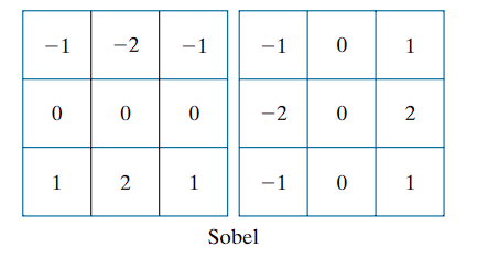
The use of a center weight of 2 offers improved noise suppression, which is critical when computing derivatives.

---

Gradient Computation and Magnitude Approximation

To compute gradient vectors:

1. Convolve the image with the appropriate pair of kernels to obtain g_x and g_y.
2. Use these to compute edge magnitude and direction.

The gradient magnitude is typically computed using:

• $M(x,y)=\sqrt{g_x^2(x,y)+g_y^2(x,y)}$

However, this computation involves squaring and square roots, which may be computationally expensive. An alternative approximation is:

• $M(x,y)\approx |g_x(x,y)|+|g_y(x,y)|$

This approximation is faster and still preserves relative intensity variations, though it introduces anisotropy—i.e., the filters become non-rotation-invariant. Nonetheless, when using Prewitt or Sobel kernels, which already produce isotropic responses only for vertical and horizontal edges, this loss of isotropy is not significant. Both these equations identical results for vertical and horizontal edges with these kernels (see Problem 10.11).

---

Kirsch Compass Operators

Prewitt and Sobel are isotropic only for vertical and horizontal edges.

So the approximate formula works well in those directions.

For general orientation detection (e.g., diagonal edges), isotropy is lost.

To handle all eight compass directions, Kirsch compass kernels (Kirsch [1971]) are used.

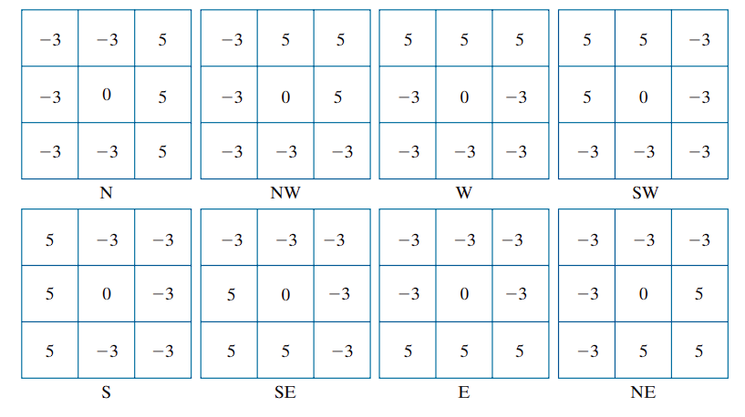
• Each kernel targets a specific compass direction (N, NE, E, etc.).
• The gradient magnitude at each pixel is taken as the maximum response from all eight kernels.
• The gradient direction is assigned based on the direction of the kernel yielding this maximum.

For instance, if the North (N) kernel produces the strongest response at a pixel, the edge direction is assigned as $0^{\circ }$. Since kernel pairs differ by $180^{\circ }$, selecting the maximum positive value ensures consistent directionality.

While the Sobel kernel treats north and south edges identically (both as vertical), the Kirsch method distinguishes them based on intensity transition direction. For example, an edge transitioning from black (0) on the left to white (1) on the right, would yield a stronger response from the N kernel, indicating a northward edge.

---

---

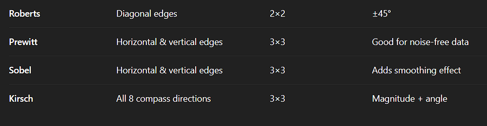
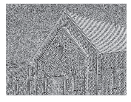
Illustration of the 2-D Gradient Magnitude and Angle

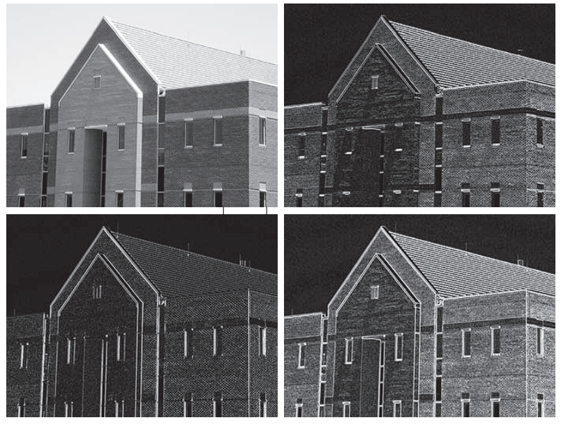Fig. 10.16

Fig illustrates the Sobel absolute value response of the two components of the gradient, g_x and g_y, as well as the gradient image formed from their sum. The directionality of the horizontal and vertical components of the gradient is clearly observed

For example:

• In (b), the roof tiles, horizontal brick joints, and horizontal window segments exhibit strong responses due to the horizontal component g_x.
• In (c), the vertical façade structures and window divisions are more prominent due to the vertical component $g_y$.

It is common to use the term edge map when referring to images that highlight edge features, such as gradient magnitude images. In these examples, the intensity values of the image were scaled to the range [0, 1] for consistency and to simplify parameter selection in edge detection algorithms.

---

Gradient Angle Image

Figure displays the gradient angle image computed using Equation

• $\theta (x,y)={\tan }^{-1}\left(\frac{g_y(x,y)}{g_x(x,y)}\right)$

Although angle images are generally not as effective for direct edge detection as magnitude images, they provide complementary information. For instance, regions with constant intensity—such as the sloping roof edge and top horizontal bands—show uniform gradient direction, as indicated by the constant pixel values in the angle image.

---

Impact of Fine Detail and Smoothing

The original image used in the example above contains high-resolution fine detail, particularly from wall bricks. While this enhances texture, it introduces undesirable noise in edge detection tasks because:

• Derivative operations amplify such high-frequency content.
• This makes it more difficult to isolate principal edges.

To mitigate this issue, the image is smoothed before gradient computation.

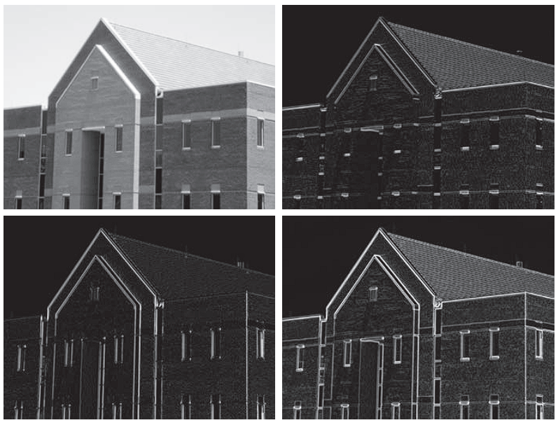Fig. 10.18

Figure presents the same sequence of images, but the original input is first processed using a 5 × 5 averaging filter. As a result:

• The influence of brick patterns is significantly reduced.
• Principal edges (e.g., structural outlines) become more dominant in the gradient responses.

---

Limitations of Sobel Kernels and Diagonal Edge Detection

The Sobel kernels do not respond strongly to edges oriented at ±45°. If diagonal edge detection is important, Kirsch compass kernels should be used.

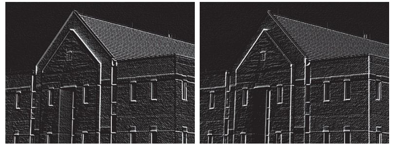
• (a) shows the response of the $+45°$ Kirsch kernel (NW direction).
• (b) shows the response of the $-45°$ Kirsch kernel (SW direction).

These figures illustrate:

• Stronger sensitivity to edges oriented along the specified diagonals.
• Weaker response to horizontal and vertical features, as expected.

Although both Kirsch kernels respond somewhat to non-diagonal edges, their stronger directional selectivity makes them particularly suited for highlighting diagonal features that Sobel kernels may miss.

---

Combining the Gradient with Thresholding

---

Edge detection can be made more selective by smoothing the image prior to computing the gradient. Another approach aimed at achieving the same objective is to threshold the gradient image.

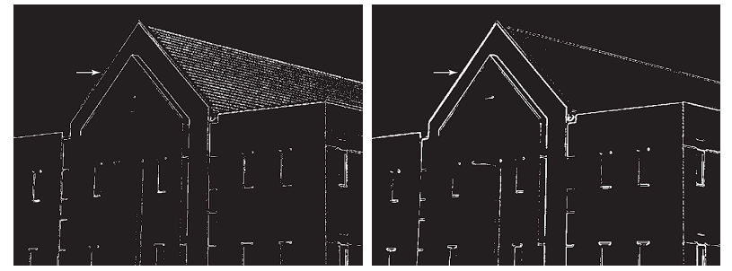
For example, (a) shows the gradient image from Fig. 10.16(d), thresholded so that pixels with values greater than or equal to 33% of the maximum value of the gradient image are shown in white, while pixels below the threshold value are shown in black.

Comparing this image with the Sobel absolute value response (Fig. 10.16(d)), we see that:

• There are fewer edges in the thresholded image.
• The edges in this image are much sharper (see, for example, the edges in the roof tile).
• On the other hand, numerous edges — such as the sloping line defining the far edge of the roof (see arrow) — are broken in the thresholded image.

When interest lies both in highlighting the principal edges and in maintaining as much connectivity as possible, it is common practice to use both smoothing and thresholding.

Figure (b) shows the result of thresholding Fig. 10.18(d), which is the gradient of the smoothed image. This result shows a reduced number of broken edges. For instance, compare the corresponding edges identified by the arrows in (a) and (b).

---

Summary

Gradient computation gives us the edge strength at every pixel — but includes everything, including noise and minor details.

Smoothing (blurring) reduces noise before computing the gradient:

• This prevents small variations (like brick textures) from being falsely detected as edges.

Thresholding removes weak edges:

• Only keeps edges where the gradient magnitude is strong enough (above a certain threshold).

• This helps highlight major edges and eliminate clutter.