Principles of Rank-Order Filtering

Consider a subimage Sₓ,ᵧ of f centered at pixel (x, y).
The subimage Sₓ,ᵧ acts as a sliding window, where the center visits every pixel (x, y) in f.
At each visited (x, y), we consider the gray values in the subimage Sₓ,ᵧ.
We rank the gray values of Sₓ,ᵧ and sort them in ascending order (from smallest to largest).
The gray value at a specified rank is taken as the gray value of the filtered image g(x, y).

Examples of ranks:

Maximum (Max Filter)
Minimum (Min Filter)
Median (Median Filter)

Explanation of the Principles

This section explains the algorithmic steps behind rank-order filtering, a class of non-linear spatial filters that, unlike linear filters (which use weighted sums), operate on the order of pixel values.

1. Sliding Window (`Sₓ,ᵧ`)

A subimage (e.g., 3×3 window) slides over the original image f.
At each position (x, y), the window is centered and gathers surrounding pixel values.

2. Gather the Pixel Values

Collect all intensity values from within Sₓ,ᵧ.
For example, in a 3×3 window, you gather 9 values.

3. Rank and Sort

Sort the gathered values in ascending order (ranking).
The sorted list provides the basis for selecting a new pixel value.

4. Pick a Value Based on Rank

The filtered value g(x, y) is chosen based on a specific rank.

Examples:

Min Filter: Pick the smallest value (first in the sorted list).
Effect: Darkens the image and expands dark regions.
Max Filter: Pick the largest value (last in the sorted list).
Effect: Brightens the image and expands bright regions.
Median Filter: Pick the middle value.
Effect: Highly effective at removing salt-and-pepper noise while preserving edges.
Example: In a 3×3 window, select the 5th value out of 9.

This process is simple yet powerful for noise reduction and edge preservation in digital image processing.

Median Filtering: Example

The subimage Sₓ,ᵧ often has an odd number of pixels, e.g., 3×3, 5×5.

As an example, we consider a 3×3 subimage Sₓ,ᵧ with gray values:

[ 1  4  7 ]
[ 7  2  3 ]
[ 4  6  6 ]

The gray values in Sₓ,ᵧ are put into an n-tuple (row-wise):
[1, 4, 7, 7, 2, 3, 4, 6, 6]
We sort these values in ascending order:
[1, 2, 3, 4, 4, 6, 6, 7, 7]
The median is the value at the center of the sorted tuple.
For 9 values, the 5th value is the median: 4
Final sorted list with the median highlighted:
[1, 2, 3, 4, **4**, 6, 6, 7, 7]

Thus, the center pixel in the filtered image g(x, y) will be 4, replacing the original value 2.

Why Median Filtering Is Effective for Denoising

If the original center pixel were a noise spike (e.g., salt noise with value 255), that extreme value would be at one end of the sorted list.
The median, being in the center, ignores such outliers.
As a result, median filtering is highly effective against impulse noise (salt-and-pepper), while still preserving edges and image structure.

alt text

Median Filtering: Elementary Properties

Example Tuples

Consider gray values in the tuple:

(30, 30, 30, 30, 30, 30, 30, 30, 30)

This represents a flat, noise-free region.
The median is: 30
Result: The image remains unchanged—no distortion or blur.

Now, adding Gaussian noise might yield:

(21, 25, 26, 27, 27, 28, 33, 35, 43)

This represents the same flat area after some moderate Gaussian noise has been added. The values are now all slightly different, scattered around the original value of 30.
The sorted version:
(21, 25, 26, 27, 27, 28, 33, 35, 43)
The median is: 27
(This differs from the original value 30)
Result: Slight deviation from true value (30), but no blurring as in averaging filters.
Observation: Median filter chooses a real value from the data, avoiding synthetic interpolation.

Now consider salt-and-pepper noise (outliers):

(0, 0, 30, 30, 30, 30, 255, 255, 255)

This represents the same flat area, but now several pixels have been corrupted with extreme “salt” (255) and “pepper” (0) noise. These are called outliers.
The sorted version:
(0, 0, 30, 30, 30, 30, 255, 255, 255)
The median is: 30
(Identical to the original value)
Result: Accurately recovers the original value.
Observation: Extreme values are pushed to the ends of the sorted list and ignored. The median filter perfectly rejects the outlier noise and recovers the original, true value. This is its greatest strength.

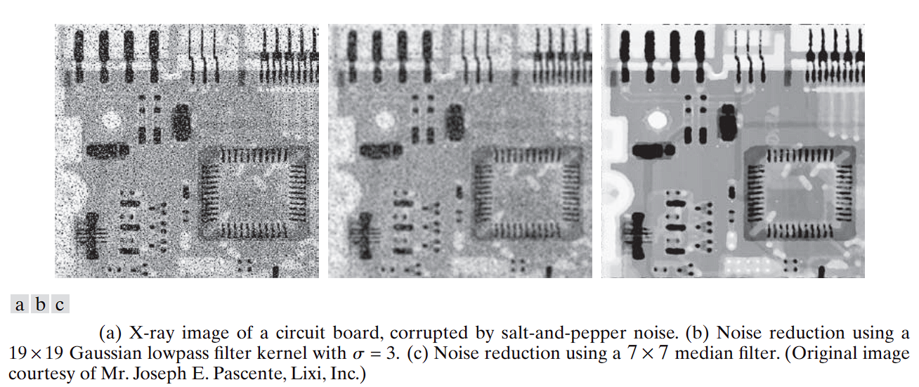
Strength (vs. Outliers): The median filter is excellent at removing salt-and-pepper noise and other impulse-like outliers. This is because the outliers are ranked at the extremes of the sorted list and are ignored when the middle value is chosen.

Weakness (vs. Gaussian Noise): The median filter is not as effective as an averaging (box) filter at removing fine-grained Gaussian noise. It will reduce the noise but may not produce as smooth a result, and it will slightly shift the true value of the pixels. Its key advantage is that it avoids the blurring that averaging filters introduce, making it much better at preserving sharp edges.

An example of The median filter’s ability to preserve sharp edges.

We consider the following 4×4 grayscale image f:

[  0   0   0   0 ]
[  0  90  90  90 ]
[  0  90  90  90 ]
[  0  90  90  90 ]

This image contains a clear vertical edge separating regions of intensity 0 and 90.

First 3×3 Subimage (Centered on Edge)

Extracted subimage:

[  0  90  90 ]
[  0  90  90 ]
[  0  90  90 ]

Corresponding 9-tuple:
(0, 90, 90, 0, 90, 90, 0, 90, 90)
Sorted:
(0, 0, 0, 90, **90**, 90, 90, 90, 90)
Median (5th value): 90
Output pixel value: 90

Second 3×3 Subimage (Also Centered on Edge)

Extracted subimage:

[  0   0   0 ]
[ 90  90  90 ]
[ 90  90  90 ]

Corresponding 9-tuple:
(0, 0, 0, 90, 90, 90, 90, 90, 90)
Sorted:
(0, 0, 0, 90, **90**, 90, 90, 90, 90)
Median (5th value): 90
Output pixel value: 90

This example illustrates what happens when a median filter window crosses a sharp intensity edge.

In both subimages, the filter’s output is either 0 or 90. When the filter’s window contains more “90” pixels than “0” pixels, the median will be 90. When it contains more “0” pixels, the median will be 0.
The median filter does not produce intermediate values (like 30 or 60), which would cause blurring in linear filters.
The median chooses an actual value from the window based on rank, not arithmetic averaging.
Edge preservation results from the filter’s tendency to snap to the majority intensity in the neighborhood. This behavior is what allows it to preserve sharp edges without blurring them. It maintains the step-like transition from one region to the next

Median Filtering: Handling Image Borders (Padding Strategies)

Example Image

Consider the following 4×4 grayscale image f:

[  0   0   0   0 ]
[  0  90  90  90 ]
[  0  90  90  90 ]
[  0  90  90  90 ]

Our goal is for the median filter to preserve edges near the boundary.

The Problem: Incomplete Filter Window Near Boundary

When applying a 3×3 median filter window centered on a pixel in the last row, part of the window lies outside the image:

[  0   90  90 ]
[  0   90  90 ]
[  ?    ?   ? ]  ← Unknown padding values

The corresponding 9-tuple is:
(0, 90, 90, 0, 90, 90, ?, ?, ?)
where ? are undefined.
To correctly compute the median, all 9 values must be known.

Desired Outcome

To preserve the apparent edge, it is desirable that the median value remains 90.
Currently, we have four known values equal to 90 and two zeros.
To have a median of 90 in a 9-element list, at least five values must be 90 or greater.
Therefore, at least one of the ? values must be 90.

Padding Strategy: Duplication (Replication)

A common and effective approach is duplicating border pixels:

Fill the unknown padding by copying the nearest valid pixels inside the image.
For this example, duplicate the last valid row:

[  0   90  90 ]
[  0   90  90 ]
[  0   90  90 ]  ← Duplicated row used for padding

The full tuple becomes:
(0, 90, 90, 0, 90, 90, 0, 90, 90)
Sorted tuple:
(0, 0, 0, 90, **90**, 90, 90, 90, 90)
Median (5th value): 90

This ensures the median filter output preserves the edge near the boundary.

Other Common Padding Methods

Zero Padding: Fill unknowns with zeros.
- In this example, would reduce median to 0, undesirably weakening the edge.
Mirror Padding: Reflect pixel values across the border.
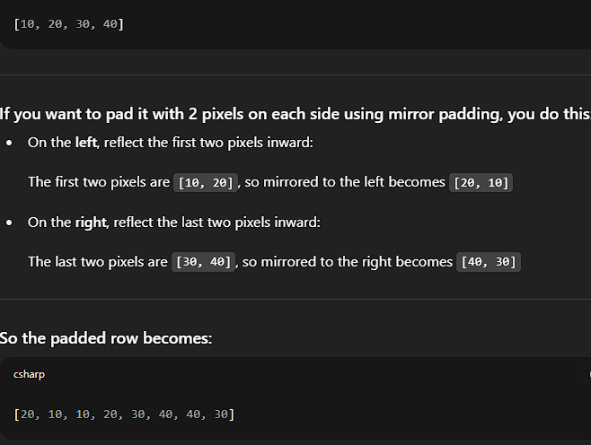
- Can also preserve edge information but with a slightly different effect.

Elementary Properties — Corner Effect

Consider the 4×4 grayscale image f:

[  0   0   0   0 ]
[  0  90  90  90 ]
[  0  90  90  90 ]
[  0  90  90  90 ]

The 3×3 Subimage at a Corner

Focus on the 3×3 subimage centered on the top-left corner pixel of the gray square:

[  0   0   0 ]
[  0  90  90 ]
[  0  90  90 ]

From this subimage, we form the 9-tuple of pixel values (row-wise):

(0, 0, 0, 0, 90, 90, 0, 90, 90)

Count of values: five 0s and four 90s.
Sorting these values:

(0, 0, 0, 0, <u>0</u>, 90, 90, 90, 90)

The median is the 5th value (middle element), which is 0.
Original center pixel value: 90
Filtered pixel value after median filtering: 0

This indicates that the corner pixel is replaced by a lower value, effectively “rounding off” or “clipping” the sharp corner of the gray square.

While the median filter is excellent at preserving straight edges without blurring, it has a known side effect near sharp convex corners.
Specifically, it tends to round off corners, smoothing or slightly distorting them.
This effect occurs because the median filter selects the middle value from a sorted neighborhood, which can shift the corner pixel’s intensity toward the background level if more background pixels surround the corner.

Example of a 3×3 median filter to a 4×4 image, incorporating mirror padding

Original 4×4 Image `f`

[  0   0   0   0 ]
[  0  90  90  90 ]
[  0  90  90  90 ]
[  0  90  90  90 ]

Step 1: Mirror Padding (6×6 Image)

To apply the median filter at all positions—including borders—we pad the image by reflecting the boundary pixels. This creates a 6×6 padded version of the original 4×4 image:

[ 0  0  0  0  0  0 ]
[ 0  0  0  0  0  0 ]
[ 0  0 90 90 90 90 ]
[ 0  0 90 90 90 90 ]
[ 0  0 90 90 90 90 ]
[ 0  0 90 90 90 90 ]

Mirror padding reflects both rows and columns outward from the edges.

Step 2: Apply 3×3 Median Filter

We now apply a 3×3 median filter centered on each pixel of the original 4×4 image (i.e., positions [1,1] to [4,4] in the padded image). For each position, the median of the corresponding 3×3 window is calculated.

Calculating Output at (1,1) — the First 90° Corner

The pixel at position (1,1) in the original 4×4 image corresponds to position (2,2) in the padded image.

3×3 window centered at (2,2):

[  0   0   0 ]
[  0  90  90 ]
[  0  90  90 ]

Flattened values:

(0, 0, 0, 0, 90, 90, 0, 90, 90)

Sorted:

(0, 0, 0, 0, **0**, 90, 90, 90, 90)

Median = 0

Thus, the corner pixel is rounded off, confirming the median filter’s natural smoothing effect at sharp transitions when using accurate mirror padding.

Final Correct Filtered Output

[  0   0   0   0 ]
[  0   0  90  90 ]
[  0  90  90  90 ]
[  0  90  90  90 ]

The upper-left corner (originally a sharp 90° transition) has now been smoothed.

Example for 3x3 Median Filtering: Thin Image Structures

We consider now as an example the 4x4 image f as follows:

[  0  90   0   0 ]
[  0  90   0   0 ]
[  0  90   0   0 ]
[  0  90   0   0 ]

Mirror padding of our example image results in:

[  0  90   0   0   0   0 ]
[  0  90   0   0   0   0 ]
[  0  90   0   0   0   0 ]
[  0  90   0   0   0   0 ]
[  0  90   0   0   0   0 ]
[  0  90   0   0   0   0 ]

Filtering result:

[  0   0   0   0 ]
[  0   0   0   0 ]
[  0   0   0   0 ]
[  0   0   0   0 ]

This example demonstrates another critical property of the median filter: its effect on small, thin details.

The image contains a thin vertical line of gray pixels (value 90) on a black background (value 0). The line is only one pixel wide.

Any pixel on the vertical line will have 3 gray pixels (90) and 6 black pixels (0) in its neighborhood.
Since 0s outnumber 90s, the median filter will output 0 at every such location.
Thus, the vertical line is entirely removed.

The median filter removes structures smaller in size than half the size of the filtering window.

For a 3×3 window, the size is 9 pixels.
Half of this is 4.5.
The vertical line has only 3 pixels in any such window → less than 4.5 → removed.

This property makes the median filter excellent at eliminating isolated noise specks but also makes it destructive to fine, thin image structures.

Morphological Image Processing

The term morphology originates from the study of shape and form.
In image processing, mathematical morphology refers to a rigorous theoretical framework for analyzing and manipulating the geometric structure of objects within digital images.
It differs fundamentally from linear filtering techniques (e.g., convolution with Gaussian kernels), which operate directly on pixel intensities. Morphological filters, in contrast, operate on shapes and structures using principles from set theory.

Mathematical morphology is based on the idea of probing an image with a small, predefined shape known as a structuring element. This concept is analogous to the kernel in linear filtering, but the operations and outcomes are entirely different due to the binary or grayscale nature of the morphological process.

Fundamental Operations

1. Erosion

Shrinks the bright regions and expands the dark ones.
Conceptually: it “erodes” away the boundaries of foreground objects.
Applications:
- Removes small bright noise.
- Separates connected objects in binary images.

2. Dilation

Expands the bright regions and shrinks the dark regions.
Conceptually: it “grows” or thickens foreground regions.
Applications:
- Fills small holes or gaps in objects.
- Bridges narrow breaks and connects disjoint components.

Composite Operations

3. Opening (Erosion followed by Dilation)

Effect:
- Removes small foreground noise.
- Preserves the overall shape and size of larger objects.
Use Case:
- Suitable for eliminating small protrusions or artifacts.

4. Closing (Dilation followed by Erosion)

Effect:
- Fills small holes or gaps within objects.
- Smooths contours without significantly altering the object area.
Use Case:
- Ideal for removing small background noise and connecting close regions.

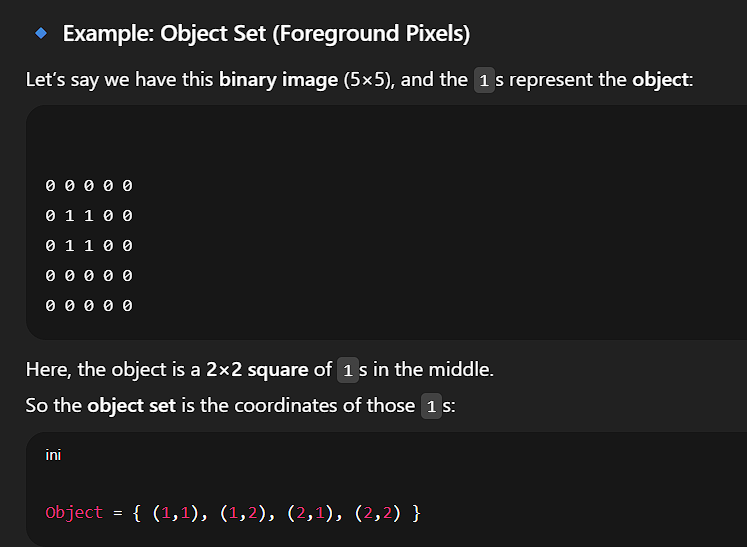
When working with images, sets in mathematical morphology represent objects in those images. In binary images, the sets in question are members of the 2-D integer space $Z^{2}$ , where each element of a set is a tuple (2-D vector) whose coordinates are the coordinates of an object (typically foreground) pixel in the image.

Grayscale digital images can be represented as sets whose components are in $Z^{3}$ . In this case, two components of each element of the set refer to the coordinates of a pixel, and the third corresponds to its discrete intensity value. Sets in higher dimensional spaces can contain other image attributes, such as color and time-varying components.

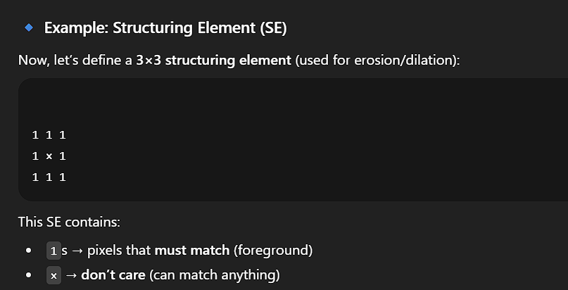
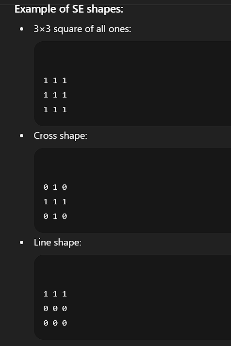
Morphological operations are defined in terms of sets. In image processing, we use morphology with two types of sets of pixels: objects and structuring elements (SEs). Typically, objects are defined as sets of foreground pixels. Structuring elements can be specified in terms of both foreground and background pixels. In addition, structuring elements sometimes contain so-called “don’t care” elements, denoted by $\times$ , signifying that the value of that particular element in the SE does not matter.

alt text

Here, the pixels with 1 (white) form a square shape — that’s the object.
The rest (pixels with 0) are the background

alt text

Because the images we work with are rectangular arrays, and sets in general are of arbitrary shape, applications of morphology in image processing require that sets be embedded in rectangular arrays. In forming such arrays, we assign a background value to all pixels that are not members of object sets.

There is an important difference between how we represent digital images and structuring elements. Digital images include a border of background pixels surrounding objects, while structuring elements do not. Structuring elements are used similarly to spatial convolution kernels, and padding operations are handled the same way as in convolution.

Set Operations

In addition to the basic definitions, the concepts of set reflection and translation are central to morphology.

Set Reflection
The reflection of a structuring element $B$ about its origin, denoted $\hat{B}$ , is defined as:

\hat{B} = {- b ∣ b \in B}

That is, if $B$ is a set of points in 2-D, then $\hat{B}$ is the set of points in $B$ whose $(x, y)$ coordinates have been replaced by $(- x, - y)$ .

Set Translation
The translation of a set $B$ by a point $z = (z_{1}, z_{2})$ , denoted $B_{z}$ , is defined as:

B_{z} = {b + z ∣ b \in B}

That is, if $B$ is a set of pixels in 2-D, then $B_{z}$ is the set of pixels in $B$ whose $(x, y)$ coordinates have been replaced by $(x + z_{1}, y + z_{2})$ .

These constructs are used to translate (slide) a structuring element over an image. At each location, a set operation is performed between the structuring element and the area of the image directly underneath it.

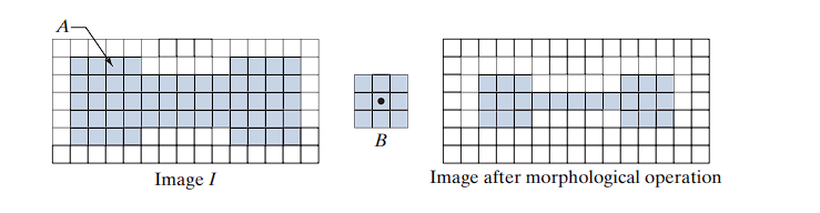
Example: Morphological Operation

Consider a binary image $I$ , containing an object $A$ and a $3 \times 3$ SE $B$ whose elements are all 1s. The background pixels (0s) are shown in white. To perform morphological erosion:

Form a new image of the same size as $I$ , initially filled with background values.
Translate $B$ over image $I$ .
At each position, if $B \subseteq A$ (i.e., $B$ is completely contained in $A$ ), mark the origin of $B$ as a foreground pixel in the new image.

If $B$ extends beyond the boundaries of $A$ , that location in the output remains background. The result is an eroded version of $A$ .

alt text

Containment Definition

When we say “the structuring element $B$ is contained in set $A$ ,” we mean specifically that the foreground elements of $B$ overlap only with elements of $A$ . This becomes important when $B$ contains background or “don’t care” elements.

The Two Main Processes

alt text

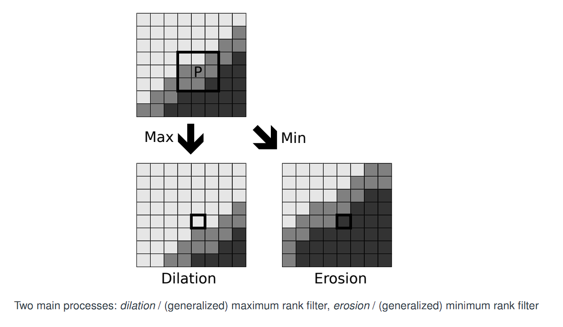
The image shows that from this starting point, we can apply one of two basic morphological operations:

The Setup (Top Image)

Original Image:
The top image is our input. It shows a grayscale image with a diagonal edge, separating a lighter region from a darker region.
Structuring Element (P):
The 3x3 black square labeled P represents the structuring element (or kernel). This is the “probe” that we slide across the image. The letter P is shown at the center of this window, which is the pixel currently being processed.

1. Dilation (The “Max” Operation)

Process:
The arrow labeled “Max” leads to the image labeled Dilation.
To calculate the new value for the center pixel P, you examine all 9 pixels inside the 3x3 window and find the maximum (brightest) value among them. This becomes the new value for the output pixel.
Connection to Rank Filters:
This is a generalized maximum rank filter, identical to the Max Filter in rank-order filtering.
Visual Result:
Look at the “Dilation” image. The center pixel P was originally a medium gray. But within its 3x3 neighborhood, there were some brighter gray pixels.
After dilation, the new center pixel becomes brighter, matching the brightest pixel in its neighborhood.
Visual Interpretation:
In the “Dilation” image, the bright region grows and the dark region shrinks. The boundary shifts up and to the left, encroaching on the dark region.
Rule:
- New pixel value = maximum in neighborhood
- Bright regions expand, dark regions contract

2. Erosion (The “Min” Operation)

Process:
The arrow labeled “Min” leads to the image labeled Erosion.
To compute the new value for P, take the minimum (darkest) value in the 3x3 window.
Connection to Rank Filters:
This is equivalent to the Min Filter in rank-order filtering.
Visual Result:
In the “Erosion” image, the dark region grows and the bright region shrinks.
The boundary moves down and to the right, and the center pixel P becomes darker.
Rule:
- New pixel value = minimum in neighborhood
- Dark regions expand, bright regions contract

Mathematical Morphology: Structuring Element

The subimage S_x,y from rank-order filtering is encoded differently in mathematical morphology,
making use of a structuring element B.

The structuring element B is defined using a set of pixels in a neighbourhood of the origin.

For example, a 3×3 structuring element has coordinates:

[ (-1,-1)  (0,-1)  (1,-1) ]
[ (-1, 0)  (0, 0)  (1, 0) ]
[ (-1, 1)  (0, 1)  (1, 1) ]

One then defines a structuring function b(x, y), which is effectively an image, via:

b(x, y) = {
    0     if (x, y) ∈ B
    -∞    otherwise
}

In rank-order filtering, the “kernel” is the full rectangular window S_x,y, and all pixels inside are treated equally.
In mathematical morphology, the structuring element B defines a specific shape inside that window. It does not need to be a solid rectangle.
The most fundamental definition of a structuring element is as a set of coordinates relative to the origin (0,0).
Examples:
- A 3×3 square:
  B = { (-1,-1), (0,-1), (1,-1), (-1,0), (0,0), (1,0), (-1,1), (0,1), (1,1) }
- A ”+” shaped element:
  B = { (0,-1), (-1,0), (0,0), (1,0), (0,1) }
This set-based approach allows arbitrary shapes, not just squares or rectangles.

Structuring Function b(x, y)

For grayscale morphology, the structuring element is defined as a function.
A flat structuring element (used in binary morphology) is defined as:

b(x, y) = {
    0     if (x, y) ∈ B
    -∞    otherwise
}

Why use 0 and -∞?
- These values interact cleanly with max (dilation) and min (erosion) operations:
  - max(pixel, -∞) returns the original pixel value.
  - min(pixel, -∞) becomes -∞, effectively removing that location from consideration.
- This formulation encodes the shape of B directly into the mathematical operation used for processing grayscale images.
Structuring elements in morphology are sets of coordinates or functions that determine how shapes in an image are probed or modified.

Mathematical Morphology: Definition of Dilation and Erosion

Our structuring function:
b(x, y) = { 0 if (x, y) ∈ B ; -∞ otherwise }

1. Dilation (f ⊕ b)

Formula:
$(f \oplus b) (x, y) = ma x_{(a, b) \in B} f (x - a, y - b) + b (a, b)$

Interpretation:

The structuring function b is flipped and centered at pixel (x, y).
For every offset (a, b) in the domain B, compute:
f(x - a, y - b) + b(a, b)
Take the maximum of these values.

Flat Structuring Element (b(a, b) = 0):

The expression simplifies to:
$(f \oplus b) (x, y) = ma x_{(a, b) \in B} f (x - a, y - b)$
This is functionally equivalent to a Max Filter over the domain B.

Plain English:
The output pixel takes on the maximum value from the region under the structuring element’s shape.

2. Erosion (f ⊖ b)

Formula:
$(f ⊖ b) (x, y) = mi n_{(a, b) \in B} f (x + a, y + b) - b (a, b)$

Interpretation:

No flipping of b.
For every offset (a, b) in the domain B, compute:
f(x + a, y + b) - b(a, b)
Take the minimum of these values.

Flat Structuring Element (b(a, b) = 0):

The expression simplifies to:
$(f ⊖ b) (x, y) = mi n_{(a, b) \in B} f (x + a, y + b)$
This is functionally equivalent to a Min Filter over the domain B.

Plain English:
The output pixel takes on the minimum value from the region under the structuring element’s shape.

⊕ denotes dilation
⊖ denotes erosion

These are standard operators in mathematical morphology and help distinguish them from simple arithmetic.

Appropriate extension at image boundary is by mirror padding. Mirror padding preserves edge continuity better than zero-padding or constant-padding.

These definitions generalize the Max/Min filters by incorporating an additional term from the structuring function b(x, y). This extra term becomes relevant in grayscale morphology and for non-flat structuring elements.

For flat structuring elements:
- Grayscale dilation reduces to a Max Filter.
- Grayscale erosion reduces to a Min Filter.
The full definitions with b(a, b) are necessary for non-flat elements, enabling more advanced morphological operations like:
- Top-hat transforms
- Morphological gradients
- Asymmetric shape probes

A detailed numerical example of how to apply the grayscale dilation operation using the simplified definition based on a flat, non-centered structuring element.

Completed Text (Slide Content)

We recall dilation of f to be:
$(f \oplus b) (x, y) = ma x_{(a, b) \in B} f ((x, y) + (a, b))$

Structuring Element B

We define the non-centered structuring element B as:

[ (0,0) (1,0) ]
[ (0,1) (1,1) ]

That is,
B = { (0,0), (1,0), (0,1), (1,1) }

This is a 2×2 block located at the top-left corner (not centered around the origin).

Input Image (with Mirror Padding)

We consider a 2×3 input image f, with 1-pixel mirror padding, resulting in a 4×5 padded image:

[ 0 | 0  1  2 | 2 ]
---------------------
[ 0 | 0  1  2 | 2 ]
[ 3 | 3  4  9 | 9 ]
---------------------
[ 3 | 3  4  9 | 9 ]

We consider the output value at the location corresponding to f(1,2) = 1

Subimage for Dilation

To compute the output, we slide the structuring element so that its (0,0) position aligns with the pixel value 1.
We then extract the 2×2 subimage that corresponds to the offsets in B:

[ 1  2 ]
[ 4  9 ]

These values come from:

(x+0, y+0) → 1
(x+1, y+0) → 2
(x+0, y+1) → 4
(x+1, y+1) → 9

Dilation Computation

Using the definition of dilation:

(f ⊕ b)(x, y) = max { f(x+a, y+b) | (a, b) ∈ B }

Substitute the extracted values:

max(1, 2, 4, 9) = 9

Final Result

The output pixel at this location (corresponding to f(1,2)) will have the new dilated value: 9

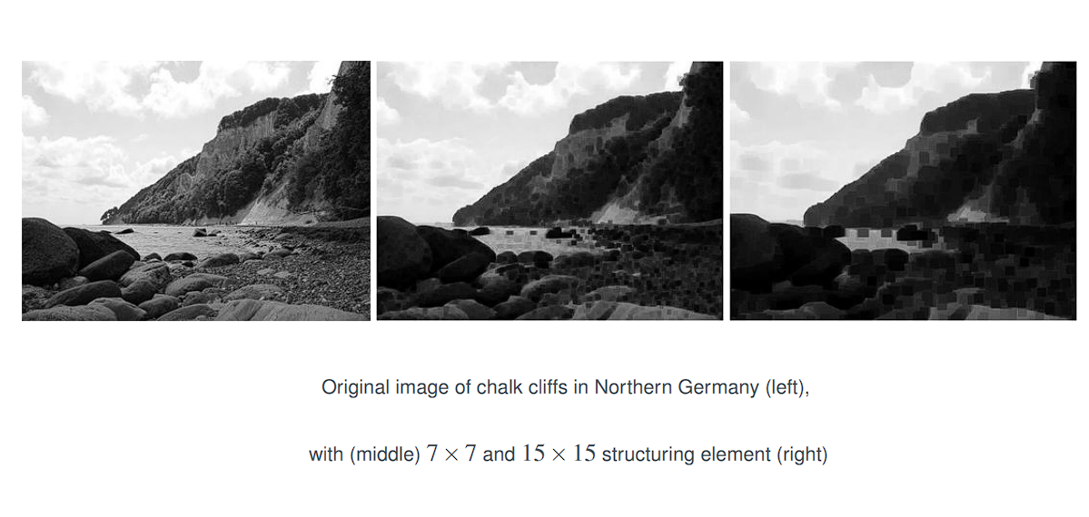
The effect of grayscale dilation with increasingly large structuring elements.

alt text

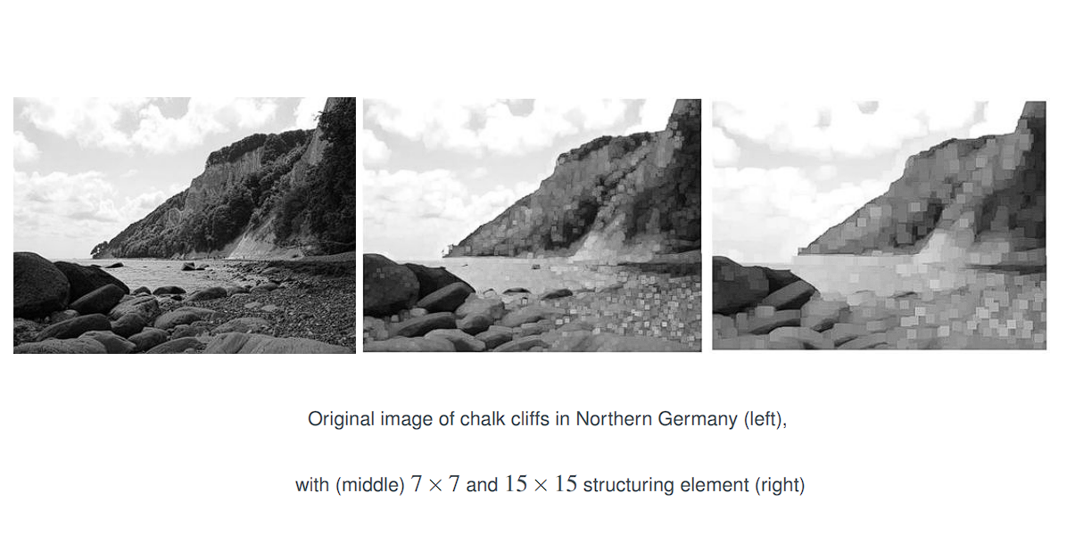
Dilation with (middle) 7x7 and 15x15 structuring element (right)

Effect on Brightness: Dilation makes bright regions in an image grow and dark regions shrink.

Effect of Structuring Element Size: The larger the structuring element, the more pronounced the morphological effect will be. A large structuring element causes a more significant loss of detail and a more dramatic alteration of the image’s geometric structures.

The effect of grayscale erosion with increasingly large structuring elements.

alt text

Erosion with (middle) 7x7 and 15x15 structuring element (right)

Effect on Brightness: Dilation makes bright regions in an image grow and dark regions shrink.

Mathematical Setup of Binary Morphology

The formal mathematical framework for Binary Morphology, where images and structuring elements are treated as sets of pixel coordinates rather than arrays of numbers.

The Universal Grid (`E`)

E = Z² denotes the set of all integer coordinate pairs (x, y) in 2D space.
It is an infinite grid, within which our finite image resides.

Let $E = Z^{2}$ be the discrete (and infinite) grid of pixels in the plane.

Images are binarized: only two values exist.
- 1: white (foreground)
- 0: black (background)

The structuring element B is a set of coordinate offsets, for example:

[ (-1,-1) (0,-1) (1,-1) ]
[ (-1, 0) (0, 0) (1, 0) ]
[ (-1, 1) (0, 1) (1, 1) ]

Let A be the set of all white pixel coordinates in the image.
Then its complement Aᶜ contains all black pixel coordinates in E.

We now interpret an image f as a set in E:
f = A ∪ Aᶜ

By convention, only the white pixels (A) are understood as the actual image.
Thus, A is a finite subset of the infinite discrete grid E.

Example:
For a 3×3 binary image with a white “X” pattern,
A = { (0,0), (2,0), (1,1), (0,2), (2,2) }
The set Aᶜ contains all other pixels in E.

Conventions

Morphological operations operate only on A.
The background (Aᶜ) is often ignored unless needed explicitly.

Finite Subset

Although E is infinite, A is always finite because images have finite dimensions.

By defining images and structuring elements as sets:

Morphological operations can be expressed using set theory:
- Union
- Intersection
- Translation
- Complement

This abstraction makes operations like binary dilation and erosion elegant, formal, and generalizable.

Geometric operations in binary morphology: translation and reflection (symmetry).

These operations are applied to sets of coordinates (e.g., structuring elements) and are foundational to morphological transformations such as dilation and erosion.

The structuring element B is a set of coordinate offsets. For example:

[ (-1,-1) (0,-1) (1,-1) ]
[ (-1, 0) (0, 0) (1, 0) ]
[ (-1, 1) (0, 1) (1, 1) ]

Translation of a Set

Definition:
For a set S ⊆ E and a vector v ∈ E, the translation of S by v is defined as:

S_{v} = s + v : s \in S

Example:
Let B be the 3×3 structuring element above. Let z = (2,2).

Then:

B_z = {
  (-1,-1)+(2,2), (0,-1)+(2,2), (1,-1)+(2,2),
  (-1, 0)+(2,2), (0, 0)+(2,2), (1, 0)+(2,2),
  (-1, 1)+(2,2), (0, 1)+(2,2), (1, 1)+(2,2)
}

Evaluating:

B_z = {
  (1,1), (2,1), (3,1),
  (1,2), (2,2), (3,2),
  (1,3), (2,3), (3,3)
}

The translated set B_z is the original shape shifted to a new center at (2,2).

Reflection (Symmetry) of a Set

Definition:
The symmetric set (or reflection through the origin) of a set B ⊆ E is defined as:

Bˢ = { x ∈ E : -x ∈ B }

In other words, for every coordinate (a, b) in B, the point (-a, -b) is in Bˢ.

Example:

Take the same 3×3 structuring element B. Let’s verify whether it is symmetric:

(-1,-1) → (-(-1), -(-1)) = (1,1) ∈ B
(1,0) → (-1,0) ∈ B
(0,1) → (0,-1) ∈ B

This holds for all elements. Therefore:

Bˢ = B

The set B is symmetric with respect to the origin.

Why Are These Operations Important?

Translation is used when we slide the structuring element over the image during dilation and erosion.
Reflection is especially important for erosion, which uses the reflected version of the structuring element.

If B is symmetric, then:

Bˢ = B, and erosion becomes simpler to compute.
We do not need to explicitly reflect B.

Binary Dilation

Let E = ℤ² be the infinite grid of all integer-coordinate pixels.
Let A ⊆ E denote the image, defined as the set of coordinates of all white (foreground) pixels.
Let B ⊆ E be the structuring element, also defined as a finite set of coordinate offsets.
Let Bˢ be the symmetric (reflected) set of B through the origin:

Bˢ = { x ∈ E : -x ∈ B }

Definition 1: Dilation via Reflected Probe

The binary dilation of A by B is defined as:

A \oplus B = z \in E : (B^{s})_{z} \cap A \neq = \emptyset

This means:

For each point z in the grid E, we:
- Reflect the structuring element B to obtain Bˢ,
- Translate Bˢ by z to get $(B^{s})_{z}$ ,
- Check whether it overlaps with the original image set A.

If the intersection is non-empty, then z is included in the dilated set.

Interpretation:
For each pixel location z, the reflected structuring element is placed so that its origin lies on z. If any part of it intersects with the foreground pixels of A, then z is marked white in the output image.

Definition 2: Dilation via Union of Translated Sets

Alternatively, binary dilation can be defined as:

A \oplus B = b \in B ⋃ A_{b}

This means:

For each vector b in the structuring element B, translate the image A by b, denoted A_b.
Take the union of all such translated sets.

Interpretation:
For every point in the structuring element B, shift the entire foreground set A accordingly and take the union of all such shifts. The resulting set is the dilated image.

The first definition is often used in theoretical proofs and formal analysis.
The second definition offers more intuitive geometric insight and is often favored in practical implementations.

Example of applying binary dilation using the filtering definition:

A \oplus B = z \in E : (B^{s})_{z} \cap A \neq = \emptyset

Input Image `A` (6×6 Grid)

We represent the image A as a binary matrix, where 1 denotes a white (foreground) pixel and 0 denotes a black (background) pixel:

A =
[ 0 0 0 0 0 0 ]
[ 0 0 0 0 0 0 ]
[ 0 0 1 1 0 0 ]
[ 0 0 1 1 0 0 ]
[ 0 0 0 0 0 0 ]
[ 0 0 0 0 0 0 ]

Set representation of foreground pixels (using 1-based indexing):

A = { (3,3), (3,4), (4,3), (4,4) }

Structuring Element B

Let B be a 3×3 square centered at the origin:

B =
[ (-1,-1) (0,-1) (1,-1) ]
[ (-1, 0) (0, 0) (1, 0) ]
[ (-1, 1) (0, 1) (1, 1) ]

B is symmetric: B = Bˢ.

Applying the Filtering Definition

For each pixel z ∈ E, we:

Translate the reflected structuring element Bˢ to be centered at z.
Check whether $(B^{s})_{z}$ has non-empty intersection with the foreground pixels of A (we check if the 3x3 window overlaps with any of the 1s in the original image A)
If the intersection is non-empty, then include z in the dilated set: z ∈ A ⊕ B(If there is an overlap, the pixel z in the output image is set to 1).

illustrates four of the 16 non-empty intersections as examples.

In each case:
- The red box indicates the center position z.
- The 3×3 window $(B^{s})_{z}$ is placed over A.
- If at least one 1 from A overlaps with the window, z is set to 1 in the result.

Let’s examine a few sample positions z:

z = (2,2):
- The 3×3 window centered here spans rows 1–3 and columns 1–3.
- Overlaps with A(3,3) = 1 → Hit → Output(2,2) = 1
z = (2,3):
- Window covers rows 1–3, columns 2–4.
- Overlaps with A(3,3) and A(3,4) → Hit → Output(2,3) = 1
z = (5,5):
- Window covers rows 4–6, columns 4–6.
- Overlaps with A(4,4) → Hit → Output(5,5) = 1
z = (1,1):
- Window covers rows 0–2, columns 0–2 (with zero-padding assumed).
- No overlap with foreground → Miss → Output(1,1) = 0

Output (Dilation Result)

The final output is a 6×6 binary image with the dilated region expanded outward by one pixel in all directions (due to the size of B):

A ⊕ B =
[ 0 0 0 0 0 0 ]
[ 0 1 1 1 1 0 ]
[ 0 1 1 1 1 0 ]
[ 0 1 1 1 1 0 ]
[ 0 1 1 1 1 0 ]
[ 0 0 0 0 0 0 ]

Mechanism: Every foreground pixel in A causes a 3×3 stamp in the output; overlapping regions form the dilated object.

Binary Dilation

The binary dilation of a set (image) $A \subseteq E$ by a structuring element $B \subseteq E$ is defined as:

A \oplus B = b \in B ⋃ A_{b}

Where:

$A_{b} = {a + b : a \in A}$ is the translation of $A$ by vector $b$ .
The result is the union of all such translations.

Equivalent Formulation

It can be shown that:

b \in B ⋃ A_{b} = a \in A ⋃ B_{a}

This implies an alternative definition:

A \oplus B = a \in A ⋃ B_{a}

That is, dilation can also be performed by translating the structuring element $B$ by each vector $a \in A$ and taking the union.

Commutativity

Because both formulations yield the same result, binary dilation is commutative:

A ⊕ B = B ⊕ A

Binary Erosion

Definition

The binary erosion of $A$ by $B$ is defined as:

A ⊖ B = z \in E : B_{z} \subseteq A

Where:

$B_{z} = {b + z : b \in B}$ is the translation of the structuring element $B$ by $z$ .
The erosion contains all points $z$ such that $B$ shifted to $z$ lies entirely within $A$ .

This is a filtering-based perspective: only positions where the entire structuring element fits inside $A$ are retained.

Equivalent (Dual) Formulation

An equivalent expression, useful for understanding the duality with dilation, is:

A ⊖ B = b \in B ⋂ A_{- b}

Where:

$A_{- b}$ denotes the translation of $A$ by $- b$ .
The erosion is the intersection of all such translated versions of $A$ .

This version is less intuitive but mathematically equivalent, and reveals erosion as a kind of “minimum” operator over translations.

Non-Commutativity

Erosion is not commutative:

A ⊖ B ≠ B ⊖ A

In fact, the results of $A ⊖ B$ and $B ⊖ A$ are often dramatically different. For example:

Eroding a large object $A$ with a small structuring element $B$ typically shrinks the object.
Eroding a small structuring element $B$ with a large object $A$ usually results in the empty set, as $B$ cannot “contain” $A$ .

Intuition

Dilation: Think of $A$ as an ink pattern and $B$ as a stamp. Dilation adds a copy of $B$ at every point in $A$ , expanding the shape.
Erosion: Think of $B$ as a stencil. Erosion keeps only those parts of $A$ where the whole stencil fits entirely within $A$ , shrinking the shape.

Algebraic Properties of Binary Dilation and Erosion

1. Commutativity of Dilation

A ⊕ B = B ⊕ A

Explanation:
The order of operands in dilation does not affect the result. Dilation is symmetric with respect to the image $A$ and the structuring element $B$ . This reflects the commutative property of vector addition.

2. Associativity of Dilation

(A ⊕ B) ⊕ C = A ⊕ (B ⊕ C)

Explanation:
Dilation is associative, meaning multiple dilations can be grouped in any way. This property allows you to combine structuring elements:

You can precompute $B \oplus C$ as a single structuring element and then apply it to $A$ .
This is similar to associativity in convolution and allows performance optimization.

3. Duality of Dilation and Erosion

A \oplus B = (A^{c} ⊖ B^{s})^{c}

Where:

$A^{c}$ is the complement of the set $A$ ,
$B^{s}$ is the reflection (or symmetric) of $B$ : $B^{s} = {- b : b \in B}$ .

Explanation:
This expresses dilation as the complement of an erosion of the background:

Dilating the foreground object $A$ is equivalent to eroding the background $A^{c}$ using the reflected structuring element $B^{s}$ , and then taking the complement again.
This is a deep and powerful theoretical property linking both operations.

Intuition:
Expanding the foreground is the same as shrinking the background.

4. Monotonicity (Increasing Property)

If $A \subseteq C$ , then:

A ⊕ B ⊆ C ⊕ B  and  A ⊖ B ⊆ C ⊖ B

Explanation:
Both dilation and erosion are increasing operators:

If $A$ is a subset of $C$ , then after applying dilation or erosion with the same structuring element $B$ , the result of $A$ ‘s operation remains a subset of $C$ ‘s.
This ensures that relative containment is preserved.

Practical Implication:
Morphological operations maintain hierarchical relationships between sets. A smaller object inside a larger one will not “escape” or change relative position due to dilation or erosion.

Composite Morphological Operation: Opening

The Opening operation is a fundamental composite morphological transformation defined by sequential application of erosion followed by dilation, both using the same structuring element.

Mathematical Definition:

A ○ B = (A ⊖ B) ⊕ B

Principle

Erosion shrinks the foreground (white) regions by removing pixels on object boundaries.
Dilation, applied to the eroded image, expands the regions again.
The result is that small objects or protrusions are removed, and only those parts of the image that can fully accommodate the structuring element are preserved.

Worked Example

Original Image A (5×5 matrix):

[ 0 0 0 0 0 ]
[ 0 1 1 1 0 ]
[ 0 1 1 1 0 ]
[ 0 1 1 1 0 ]
[ 0 0 0 0 0 ]

This represents a 3×3 square of 1s centered in a 5×5 image.

Structuring Element B: a 3×3 square.

Step 1: Erosion `A ⊖ B`

Rule: A pixel remains 1 in the output if and only if the structuring element B, when centered at that pixel, fits entirely within the foreground (1-valued) region of the input image.

Result:

[ 0 0 0 0 0 ]
[ 0 0 0 0 0 ]
[ 0 0 1 0 0 ]
[ 0 0 0 0 0 ]
[ 0 0 0 0 0 ]

Only the center pixel (2,2) meets the criterion. At all other positions, the structuring element would extend beyond the original object.

Step 2: Dilation `(A ⊖ B) ⊕ B`

Rule: A pixel becomes 1 if any part of the structuring element overlaps with a 1 in the input image (the eroded result).

Interpretation: This step effectively places the structuring element centered at every 1 in the eroded image. Since there is only one such 1 (at the center), the result is a replication of the structuring element centered at that location.

Result:

[ 0 0 0 0 0 ]
[ 0 1 1 1 0 ]
[ 0 1 1 1 0 ]
[ 0 1 1 1 0 ]
[ 0 0 0 0 0 ]

Conclusion and Key Property

Notice that the final result is identical to the original image. This demonstrates the first essential property of opening:

White structures that are at least the same size and shape as the structuring element are preserved exactly.

Use Case

Opening is widely used in:

Noise removal (e.g., salt noise).
Preprocessing for shape analysis.
Segmenting meaningful components in cluttered binary images.

Morphological Composite Operation: Opening (Example 2)

Input Image A (6×6):

A binary image containing a somewhat irregular shape with protrusions and thin connections:

[ 0 0 0 0 0 0 ]
[ 0 1 1 1 0 0 ]
[ 0 1 1 1 1 0 ]
[ 0 1 1 1 1 0 ]
[ 0 1 0 1 0 0 ]
[ 0 0 0 0 0 0 ]

Structuring Element B:

A 3×3 square:

[ 1 1 1 ]
[ 1 1 1 ]
[ 1 1 1 ]

Step 1: Erosion `A ⊖ B`

Rule: A pixel in the output is 1 if the entire structuring element B fits within the foreground (1s) of A when centered at that pixel.

Erosion Output:

[ 0 0 0 0 0 0 ]
[ 0 0 0 0 0 0 ]
[ 0 0 0 0 0 0 ]
[ 0 0 1 0 0 0 ]
[ 0 0 0 0 0 0 ]
[ 0 0 0 0 0 0 ]

Step 2: Dilation `(A ⊖ B) ⊕ B`

Rule: Each foreground pixel in the erosion output is expanded by placing the structuring element B centered at that location.

Since the input has a single 1 at (4,3), the dilation result will be a 3×3 block centered at that position.

Dilation Output (Final Result of Opening):

[ 0 0 0 0 0 0 ]
[ 0 1 1 1 0 0 ]
[ 0 1 1 1 0 0 ]
[ 0 1 1 1 0 0 ]
[ 0 0 0 0 0 0 ]
[ 0 0 0 0 0 0 ]

Structures smaller than the structuring element are removed and not preserved.

This means any connected component in the image that cannot fully contain the structuring element is eliminated during the erosion step.

Geometric Analogy: Bays and Coastlines

This analogy helps conceptualize the morphological effect of opening.

“White bays are opened”:
- Narrow inlets or gaps in objects (e.g., U-shapes) are widened as erosion removes the surrounding structure.
“White coasts are reduced to clear coastlines”:
- Irregular edges, narrow protrusions, and fine extensions are removed, leaving behind a cleaner and smoother shape.

The result is akin to smoothing a jagged coastline—eroding sharp features and then gently expanding what remains.

Morphological Composite Operation: Closing

1. Definition of Closing

The Closing operation is the dual of Opening and is defined as follows:

Principle: Apply dilation first, followed by erosion.
Formula:

A • B = (A ⊕ B) ⊖ B

2. Example Calculation

Input Image `A` (7×7):

A binary image containing a 3×3 square of foreground pixels (1s) surrounded by background pixels (0s):

[ 0 0 0 0 0 0 0 ]
[ 0 0 0 0 0 0 0 ]
[ 0 0 1 1 1 0 0 ]
[ 0 0 1 1 1 0 0 ]
[ 0 0 1 1 1 0 0 ]
[ 0 0 0 0 0 0 0 ]
[ 0 0 0 0 0 0 0 ]

Structuring Element `B`:

A standard 3×3 square:

[ 1 1 1 ]
[ 1 1 1 ]
[ 1 1 1 ]

Step 1: Dilation (`A ⊕ B`)

Rule: Dilate the image by expanding each foreground pixel by the shape of the structuring element.
Effect: The 3×3 square expands outward by one pixel in all directions.
Expected Result: A 5×5 square of 1s centered within the 7×7 grid.

Dilation Output:

[ 0 1 1 1 1 1 0 ]
[ 0 1 1 1 1 1 0 ]
[ 0 1 1 1 1 1 0 ]
[ 0 1 1 1 1 1 0 ]
[ 0 1 1 1 1 1 0 ]
[ 0 1 1 1 1 1 0 ]
[ 0 0 0 0 0 0 0 ]

(Note: The example image shows a 6×5 shape, which appears to be a typographical inconsistency. The conceptual operation results in a 5×5 square.)

Step 2: Erosion (`(A ⊕ B) ⊖ B`)

Rule: Erode the dilated image using the same structuring element.
Effect: The object shrinks by one pixel from all sides, reversing the expansion but preserving any holes filled during dilation.
Expected Result: The original 3×3 square restored, with small holes filled.

Erosion Output:

[ 0 0 0 0 0 0 0 ]
[ 0 0 1 1 1 0 0 ]
[ 0 0 1 1 1 0 0 ]
[ 0 0 1 1 1 0 0 ]
[ 0 0 0 0 0 0 0 ]
[ 0 0 0 0 0 0 0 ]
[ 0 0 0 0 0 0 0 ]

Example

Given:

Input image A is an 8×7 binary matrix.
Structuring element B is a standard 3×3 square.

Input Image `A` (8×7):

[ 0 0 0 0 0 0 0 ]
[ 0 0 0 0 0 0 0 ]
[ 0 0 1 1 0 0 0 ]
[ 0 0 1 1 1 0 0 ]
[ 0 0 1 1 1 0 0 ]
[ 0 0 1 0 1 0 0 ]
[ 0 0 0 0 0 0 0 ]
[ 0 0 0 0 0 0 0 ]

Structuring Element `B`:

A 3×3 square structuring element:

[ 1 1 1 ]
[ 1 1 1 ]
[ 1 1 1 ]

Step 1: Dilation (`A ⊕ B`)

Dilation expands all foreground pixels by one pixel in every direction.
Small gaps and holes are filled during this process.
The 1-pixel hole at position (3,5) is filled because the structuring element overlaps with surrounding foreground pixels.
The gap at (6,4) is similarly filled due to expansion and merging.
The resulting shape forms a solid block spanning rows 2 to 7 and columns 2 to 6, i.e., a 6×5 block of ones.

Dilated Image:

[ 0 0 0 0 0 0 0 ]
[ 0 0 1 1 1 1 0 ]
[ 0 0 1 1 1 1 0 ]
[ 0 0 1 1 1 1 0 ]
[ 0 0 1 1 1 1 0 ]
[ 0 0 1 1 1 1 0 ]
[ 0 0 1 1 1 1 0 ]
[ 0 0 0 0 0 0 0 ]

Step 2: Erosion (`(A ⊕ B) ⊖ B`)

Erosion shrinks the shape by removing pixels from the boundary.
Using the 3×3 structuring element, the 6×5 block is eroded to a smaller 4×3 block.
The top-left corner of this eroded block is at position (3,3) in the image.
This results in a solid 4×3 block of ones, smoothing the boundaries and removing small protrusions.

[ 0 0 0 0 0 0 0 ]
[ 0 0 0 0 0 0 0 ]
[ 0 0 1 1 1 0 0 ]
[ 0 0 1 1 1 0 0 ]
[ 0 0 1 1 1 0 0 ]
[ 0 0 1 1 1 0 0 ]
[ 0 0 0 0 0 0 0 ]
[ 0 0 0 0 0 0 0 ]

Interpretation and Properties

White “bays” are “closed”: The initial dilation fills in narrow inlets and small holes in the shape, effectively “closing” these bays.
White “coasts” are completed to clear “coastlines”: The closing operation smooths the contour by filling gaps and completing edges, producing a simpler and more regular shape without internal holes or irregular boundaries.

Properties of Closing

Fills small holes: The initial dilation expands the object, closing small gaps or holes. The subsequent erosion removes the expansion except where holes were filled, preserving these areas.
Smooths contours: Closing smooths object boundaries from the inside by bridging narrow breaks and filling small inlets or bays.
Preserves large background structures: Only small black holes or gaps are filled. Large holes remain unaffected if they cannot accommodate the structuring element.

Formal Property:

Black structures (background holes) that are at least the size and shape of the structuring element are preserved exactly.

Agney's Digital Garden

📁 Explorer

Lecture 06 - Morphological Operations

Principles of Rank-Order Filtering

Explanation of the Principles

1. Sliding Window (Sₓ,ᵧ)

2. Gather the Pixel Values

3. Rank and Sort

4. Pick a Value Based on Rank

Examples:

Median Filtering: Example

Why Median Filtering Is Effective for Denoising

Median Filtering: Elementary Properties

Example Tuples

First 3×3 Subimage (Centered on Edge)

Second 3×3 Subimage (Also Centered on Edge)

Median Filtering: Handling Image Borders (Padding Strategies)

Example Image

The Problem: Incomplete Filter Window Near Boundary

Desired Outcome

Padding Strategy: Duplication (Replication)

Other Common Padding Methods

Elementary Properties — Corner Effect

The 3×3 Subimage at a Corner

Example of a 3×3 median filter to a 4×4 image, incorporating mirror padding

Original 4×4 Image f

Step 1: Mirror Padding (6×6 Image)

Step 2: Apply 3×3 Median Filter

Calculating Output at (1,1) — the First 90° Corner

Final Correct Filtered Output

Example for 3x3 Median Filtering: Thin Image Structures

Morphological Image Processing

Fundamental Operations

1. Erosion

2. Dilation

Composite Operations

3. Opening (Erosion followed by Dilation)

4. Closing (Dilation followed by Erosion)

Set Operations

Example: Morphological Operation

Containment Definition

The Two Main Processes

The Setup (Top Image)

1. Dilation (The “Max” Operation)

2. Erosion (The “Min” Operation)

Mathematical Morphology: Structuring Element

Structuring Function b(x, y)

Mathematical Morphology: Definition of Dilation and Erosion

1. Dilation (f ⊕ b)

2. Erosion (f ⊖ b)

Completed Text (Slide Content)

Structuring Element B

Input Image (with Mirror Padding)

Subimage for Dilation

Dilation Computation

Final Result

The effect of grayscale dilation with increasingly large structuring elements.

The effect of grayscale erosion with increasingly large structuring elements.

Mathematical Setup of Binary Morphology

The Universal Grid (E)

Conventions

Finite Subset

Geometric operations in binary morphology: translation and reflection (symmetry).

Translation of a Set

Reflection (Symmetry) of a Set

Why Are These Operations Important?

Binary Dilation

Definition 1: Dilation via Reflected Probe

Definition 2: Dilation via Union of Translated Sets

Input Image A (6×6 Grid)

Structuring Element B

Applying the Filtering Definition

Output (Dilation Result)

Binary Dilation

Equivalent Formulation

Commutativity

Binary Erosion

Definition

Equivalent (Dual) Formulation

Non-Commutativity

1. Sliding Window (`Sₓ,ᵧ`)

Original 4×4 Image `f`

The Universal Grid (`E`)

Input Image `A` (6×6 Grid)

Step 1: Erosion `A ⊖ B`

Step 2: Dilation `(A ⊖ B) ⊕ B`

Step 1: Erosion `A ⊖ B`

Step 2: Dilation `(A ⊖ B) ⊕ B`

Input Image `A` (7×7):

Structuring Element `B`:

Step 1: Dilation (`A ⊕ B`)

Step 2: Erosion (`(A ⊕ B) ⊖ B`)

Input Image `A` (8×7):

Structuring Element `B`:

Step 1: Dilation (`A ⊕ B`)

Step 2: Erosion (`(A ⊕ B) ⊖ B`)