Lecture 07 - Image Compression & Frequency Domain

ADVANCED TECHNIQUES FOR EDGE DETECTION

Review of Second-Order Derivatives in Image Processing

The Laplacian Operator

The discrete Laplacian of an image function $f(x,y)$ is denoted as:

${\nabla }^{2}f(x,y)$

It is defined as the sum of the second-order partial derivatives in the horizontal and vertical directions:

${\nabla }^{2}f(x,y)=\frac{{\partial }^{2}f}{\partial x^2}+\frac{{\partial }^{2}f}{\partial y^2}$

The operator is not biased toward any direction — it gives equal weight to changes in x and y. That’s why it’s symmetric

A gradient points in a direction.

The Laplacian is scalar: it gives you a single value that says whether the intensity is peaking, dipping, or flat — but not which way. It doesn’t tell you the direction of change — only that there is a curvature

• The Laplacian operator is symmetric and non-directional.

---

Discrete Approximations of Second Derivatives

• The second derivative in the $x$-direction can be approximated by the discrete kernel:

$\frac{{\partial }^{2}f}{\partial x^2}\approx [1,-2,1]$

• The second derivative in the $y$-direction can be approximated by the column kernel:

$\frac{{\partial }^{2}f}{\partial y^2}\approx \left[\begin{array}{c}1\\ -2\\ 1\end{array}\right]$

These kernels represent discrete second differences, obtained by convolving a first difference kernel with its inverse.

---

Construction of Laplacian Kernels

By combining the two kernels, the Laplacian operator can be represented by convolution masks.

1. 4-Connectivity Laplacian Mask
   This mask considers only the immediate horizontal and vertical neighbors:

$\left[\begin{array}{ccc}0& 1& 0\\ 1& -4& 1\\ 0& 1& 0\end{array}\right]$

2. 8-Connectivity Laplacian Mask
   This mask includes diagonal neighbors as well:

$\left[\begin{array}{ccc}1& 1& 1\\ 1& -8& 1\\ 1& 1& 1\end{array}\right]$

---

Interpretation and Applications

• The Laplacian is a scalar operator measuring the sum of curvatures along the two principal axes.
• It responds strongly at points of rapid intensity change, especially at edges, producing zero-crossings at edge locations.
• In regions of constant intensity or constant slope (ramps), the Laplacian output is zero.

Applications:

• Edge Detection: Locating edges by identifying zero-crossings in the Laplacian-filtered image.
• Image Sharpening: Enhancing fine details by subtracting a scaled Laplacian from the original image, accentuating edges and textures.

Zero-crossings of the second-order derivatives correspond to the precise locations of edges in an image. However, derivative-based methods are highly sensitive to noise.

• Sensitivity to Noise: Derivative operations amplify noise because they involve computing differences between neighboring pixels.

• The second derivative is even more sensitive since it represents differences of differences.

---

Using zero crossings for edge detection

The Marr-Hildreth Edge Detector: Principle and Implementation

The edge-detection methods previously discussed rely on simple filtering operations using fixed-size convolution kernels. While computationally efficient, these basic methods do not account for edge characteristics or image noise.

The Marr-Hildreth method, introduced by Marr and Hildreth (1980), is one of the earliest attempts to embed a deeper understanding of visual perception into computational edge detection. The two central insights motivating their approach are:

1. Scale Matters: Intensity transitions are not independent of scale. Therefore, edge detection requires analyzing the image at different resolutions using filters of varying size.
2. Zero-Crossings as Edges: A sudden change in intensity manifests as a peak or trough in the first derivative, or equivalently, as a zero-crossing in the second derivative.

Desired Properties of an Edge Detector

Marr and Hildreth argued that an effective edge-detection operator should:

• Be a differential operator that approximates the first or second derivative at each image point.
• Be tunable in scale, enabling the detection of both fine detail and broad, smooth transitions.

---

The Laplacian of Gaussian (LoG) Operator

The Marr-Hildreth detector uses the Laplacian of Gaussian (LoG) operator, defined as:

$$\text{LoG}(x,y)={\nabla }^{2}G(x,y)$$

where ${\nabla }^2$ is the Laplacian operator and $G(x,y)$ is a 2D Gaussian function:

$$G(x,y)=e^{-\frac{x^2+y^2}{2{\sigma }^2}}$$

Applying the Laplacian to the Gaussian yields:

$${\nabla }^{2}G(x,y)=\left(\frac{x^2+y^2-2{\sigma }^2}{{\sigma }^4}\right)e^{-\frac{x^2+y^2}{2{\sigma }^2}}$$

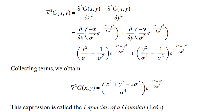
This function is radially symmetric and isotropic.

Visualization and Structure of the Laplacian of Gaussian (LoG) Operator

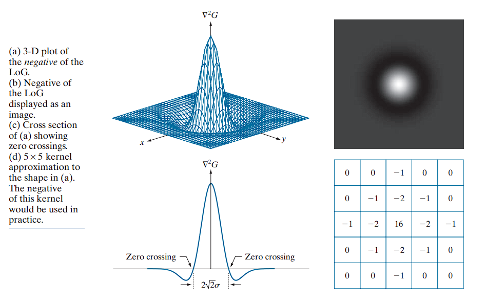
(a) 3D Surface Plot of the LoG Function

This plot presents the continuous LoG function, denoted as ${\nabla }^{2}G(x,y)$.

• “Mexican Hat” Shape: A central positive peak surrounded by a negative ring, resembling a sombrero.
• Radial Zero-Crossings: Occur at points where $x^2+y^2=2{\sigma }^2$, forming a circle of radius $\sqrt{2}\sigma$.
• Decay to Zero: The function approaches zero at distances far from the center.

(b) Grayscale Image of the LoG

This is the LoG filter displayed as a grayscale image, where brightness corresponds to function amplitude.

Interpretation:

• White Center: Represents the positive peak.
• Dark Ring: Denotes the surrounding negative trough.
• Gray Background: Indicates areas where the LoG value is approximately zero.

---

(c) 1D Cross-Section (Profile View)

This subplot shows a 1D slice through the center of the 3D LoG surface.

Observations:

• Positive Central Peak: The maximum of the function.
• Symmetric Negative Troughs: Represent adjacent regions of intensity decrease.
• Zero-Crossings: Critical points where the function transitions from positive to negative. These define potential edge locations and occur approximately at $x=\pm \sqrt{2}\sigma$.

---

(d) 5×5 Discrete LoG Kernel Approximation

This kernel is a sampled and quantized approximation of the continuous LoG function, used for convolution in digital image processing.

The negative of this kernel would be used in practice. This is specifically for image sharpening

Example Kernel:

[  0   0   1   0   0 ]
[  0   1   2   1   0 ]
[  1   2 -16   2   1 ]
[  0   1   2   1   0 ]
[  0   0   1   0   0 ]

Properties:

• Central Positive Value (16): Represents the peak of the LoG.
• Surrounding Negative Values: Capture the negative trough.
• Zero Sum: The kernel coefficients should sum to zero to suppress constant regions:

Sharpening Formula

Let $f$ be the original image and ${\nabla }^{2}f$ the Laplacian-filtered image.

The standard sharpening operation is:

$$g_{\text{sharp}}=f-k\cdot ({\nabla }^{2}f)$$

If using the LoG filter, the sharpening becomes:

$$g_{\text{sharp}}=f-k\cdot ({\nabla }^{2}G\ast f)$$

This can be expressed as a convolution:

$$g_{\text{sharp}}=(\delta -k\cdot {\nabla }^{2}G)\ast f$$

Where $\delta$ is the impulse kernel (identity).

Equivalently:

$$g_{\text{sharp}}=f+k\cdot (-{\nabla }^{2}G\ast f)$$

This final form clarifies the importance of using the negative LoG: the sharpening effect is achieved by adding the detail signal extracted by the negative Laplacian of Gaussian back to the original image.

---

Properties and Implementation of the LoG

• The Gaussian component smooths the image, attenuating high-frequency noise.
• The Laplacian detects areas of rapid intensity change (edges).
• Because the Laplacian is isotropic, it responds equally to edges in all directions.
• The LoG kernel has zero mean, ensuring a zero response in constant-intensity regions.

To approximate the LoG in practice:

1. Sample the continuous LoG expression to form a discrete kernel of appropriate size.
2. Alternatively, compute it by convolving a Gaussian-smoothed image with a discrete Laplacian kernel (e.g., a $3\times 3$ mask).

---

Marr-Hildreth Edge Detection Algorithm

The algorithm proceeds in three main steps:

1. Gaussian Smoothing
   Convolve the input image $f(x,y)$ with a Gaussian kernel of size $n\times n$, sampled from the expression for $G(x,y)$.

2. Apply the Laplacian Operator
   Convolve the smoothed image with a Laplacian kernel (e.g., a $3\times 3$ mask) to compute the second derivative.

3. Detect Zero-Crossings
   For each pixel $p$, examine its $3\times 3$ neighborhood in the filtered image. A zero-crossing occurs at $p$ if the signs of two opposing neighbors differ and their absolute difference exceeds a predefined threshold.

The full process can be expressed as:

$$g(x,y)={\nabla }^2[G(x,y)\ast f(x,y)]$$

Or, equivalently:

$$g(x,y)=[{\nabla }^{2}G(x,y)]\ast f(x,y)$$

---

Kernel Size Selection

To determine an appropriate kernel size for the Gaussian filter:

• Use a kernel of size $L\times L$, where $L=\lceil 6\sigma \rceil$
• Ensure $L$ is an odd integer for symmetry.
• This ensures that the tail of the Gaussian (beyond $3\sigma$) is negligible.

Using a kernel smaller than this will truncate the LoG and compromise edge detection performance.

---

Thresholding for Edge Confirmation

To avoid false detections due to minor variations or noise:

• Apply a threshold to the difference between positive and negative values across a zero-crossing.
• Only mark a pixel as an edge if this difference exceeds the threshold.

This step helps suppress insignificant or noisy zero-crossings.

---

Zero-Crossing Detection Procedure

For each pixel $p$ in the LoG-filtered image, we apply a two-part test using a $3\times 3$ neighborhood centered on $p$:

1. Sign Change Condition

We test for the presence of a zero-crossing based on the sign of ${\nabla }^{2}G(x,y)$ (the Laplacian of Gaussian).

Procedure:

• Consider the four pairs of opposite neighbors around $p$ in the $3\times 3$ mask:
  • Horizontal: Left and right
  • Vertical: Top and bottom
  • Diagonal (/): Top-right and bottom-left
  • Diagonal (\): Top-left and bottom-right

Condition:

• A sign change is detected if, in any of the four pairs:
  • One pixel has a positive LoG value and the other has a negative value.

This indicates that the Laplacian function crosses zero at or near pixel $p$.

---

2. Threshold Condition

The sign change condition alone is too sensitive and may detect minor fluctuations due to noise. To suppress such false positives, we introduce a threshold test.

Procedure:

• For any pair where a sign change is found:
  • Compute the absolute difference between the pixel values: $$|{\nabla }^{2}G(x_1,y_1)-{\nabla }^{2}G(x_2,y_2)|$$
• Compare this value to a user-defined threshold.

Condition:

• The difference must exceed a threshold $T$, i.e., $$|{\text{value}}_1-{\text{value}}_2|>T$$
• Only then is the sign change considered significant.

---

3. Final Decision

A pixel $p$ is marked as a zero-crossing pixel (i.e., part of an edge) if and only if both of the following conditions are satisfied:

• There is a sign change in at least one of the four opposite pixel pairs.
• The absolute difference of the pair exceeds the threshold.

This two-part test improves the robustness of the Marr-Hildreth detector by ensuring that only meaningful zero-crossings (likely corresponding to edges) are preserved.

---

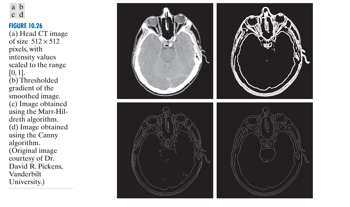
Example

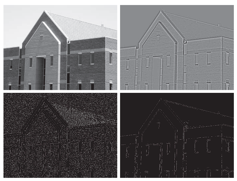
Applying the Marr-Hildreth edge detection method to a grayscale building image.

• (a): Original building image.
• (b): Result of applying Steps 1 and 2 of the Marr-Hildreth algorithm.
• (c): Zero-crossing result with a zero threshold.
• (d): Zero-crossing result with a positive threshold (4% of maximum LoG value).

Parameters

• $s=4$: Standard deviation of the Gaussian used for smoothing. This value corresponds to approximately 0.5% of the short dimension of the image.
• $n=25$: Size of the LoG mask used to ensure it adequately captures the Gaussian profile (as required by the size condition).

(b) Output of Steps 1 and 2

• The Laplacian of Gaussian (LoG) is applied using the given $s$ and $n$ values.
• Gray tones in the image result from intensity scaling for visualization.
• This output is the input for zero-crossing detection.

(c) Zero-Crossings with Zero Threshold

• Threshold: 0
• Method: A $3\times 3$ neighborhood-based approach is used to identify zero-crossings.
• Result: Many closed-loop edges appear, a phenomenon known as the “spaghetti effect”.
  • These loops often do not correspond to real object boundaries.
  • This is a major limitation of using a zero threshold.

(d) Zero-Crossings with Threshold = 4% of Maximum LoG Value

• Threshold: $0.04\times \max (\text{LoG})$

• Result:

  • Major structural edges are preserved (e.g., outlines of windows, walls).
  • Irrelevant features (e.g., bricks and tiles) are effectively filtered out.
  • This improved performance is difficult to achieve with gradient-based edge detectors.

• Another important consequence of using zero crossings for edge detection is that the resulting edges are 1 pixel thick - 1-pixel-thick edges simplify subsequent steps such as edge linking and region segmentation.

---

Huertas & Medioni’s Subpixel Method

If the accuracy of the zero-crossing locations found using the Marr-Hildreth edge-detection method is inadequate in a particular application, then a technique proposed by Huertas and Medioni for finding zero crossings with subpixel accuracy can be employed.

• Fits a smooth curve to better pinpoint the edge location
• Best for applications needing very precise edge detection, like medical imaging

---

Approximate the Laplacian of Gaussian (LoG) function by a Difference of Gaussians (DoG):

$$D(x,y)=\frac{1}{2\pi {\sigma }_1^2}{e}^{-\frac{x^2+y^2}{2{\sigma }_1^2}}-\frac{1}{2\pi {\sigma }_2^2}{e}^{-\frac{x^2+y^2}{2{\sigma }_2^2}}$$

where ${\sigma }_2>{\sigma }_1$.

---

Relationship to Human Vision

Experimental results suggest that certain channels in the human vision system are selective for both orientation and frequency. These can be modeled using above equation with a ratio of standard deviations of:

• $1.75:1$ — matches physiological observations.
• $1.6:1$ — provides a closer engineering approximation to the LoG function (Marr and Hildreth, 1980).

---

Matching Zero Crossings

To ensure that the LoG and DoG have the same zero crossings, the value of $\sigma$ for the LoG must satisfy:

$${\sigma }^2=\frac{{\sigma }_1^2{\sigma }_2^2}{{\sigma }_2^2-{\sigma }_1^2}\ln \left(\frac{{\sigma }_2}{{\sigma }_1}\right)$$

Although their zero crossings match when this equation is satisfied, their amplitude scales will differ. To make them comparable, both functions are scaled so that they have the same value at the origin.

---

The Canny Edge Detector

The Canny edge detector (Canny, 1986) is a multi-stage algorithm designed to produce optimal edge detection results based on three primary objectives:

1. Low error rate — Detect all true edges and avoid spurious responses.
2. Good localization — Edge points should be as close as possible to the true edge position.
3. Single response per edge — Only one pixel should be marked for each true edge point.

Canny expressed these criteria mathematically and derived an optimal detector for 1-D step edges corrupted by additive white Gaussian noise. The result showed that a good approximation is obtained by the first derivative of a Gaussian:

$$\frac{d}{dx}\left(e^{-\frac{x^2}{2{\sigma }^2}}\right)=-\frac{x}{{\sigma }^2}{e}^{-\frac{x^2}{2{\sigma }^2}}$$

This function performs within approximately 20% of the optimal numerical solution, a difference generally imperceptible in practical applications.

---

Extension to 2-D

For 2-D images, the process is applied in the direction of the edge normal. Since this direction is not known in advance, the method approximates it by:

1. Smoothing the image with a 2-D Gaussian function: $$G(x,y)=e^{-\frac{x^2+y^2}{2{\sigma }^2}}$$
2. Convolving the image with $G(x,y)$: $$f_s(x,y)=f(x,y)\ast G(x,y)$$
3. Computing the gradient magnitude and angle: $$M_s(x,y)=\sqrt{g_x^2(x,y)+g_y^2(x,y)}$$ $$\alpha (x,y)={\tan }^{-1}\left(\frac{g_y(x,y)}{g_x(x,y)}\right)$$ where $g_x=\frac{\partial f_s}{\partial x}$ and $g_y=\frac{\partial f_s}{\partial y}$.

---

Non-Maxima Suppression

The gradient magnitude image $M_s(x,y)$ typically contains wide ridges around local maxima. To produce thin edges, we apply non-maxima suppression.

• The goal of non-maximum suppression is to thin these ridges down to single-pixel-wide lines, preserving only the pixels that are the true “peak” of the ridge.

The core idea is : “An edge pixel should only survive if its gradient magnitude is greater than its two neighbors in the direction perpendicular to the edge.” Since the gradient direction is always perpendicular to the edge, this is the same as saying:

• “A pixel p is an edge pixel only if its gradient magnitude is greater than the magnitudes of its two neighbors along the gradient direction.”

Discrete Edge Orientations

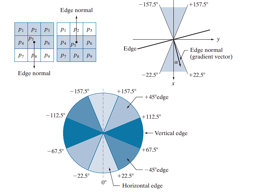
In a $3\times 3$ neighborhood, the edge normal (i.e., gradient vector direction) is quantized into four orientations:

• Horizontal ($0^{\circ }$)
• Vertical ($90^{\circ }$)
• $+45^{\circ }$
• $-45^{\circ }$

For example:

• A horizontal edge corresponds to edge normals in the ranges: $$-22.5^{\circ }\le \alpha (x,y)\le 22.5^{\circ }\text{or}157.5^{\circ }\le \alpha (x,y)\le -157.5^{\circ }$$
• Similar angular ranges define the remaining three orientations.

Algorithm

Let $d_1,d_2,d_3,d_4$ denote the four possible edge directions (horizontal, $-45^{\circ }$, vertical, $+45^{\circ }$).
For a pixel centered at $(x,y)$:

1. Find the closest orientation $d_k$ to the gradient direction $\alpha (x,y)$.
2. Let $K=f_s(x,y)$.
   • Compare $K$ with its two neighbors along direction $d_k$.
   • If $K$ is smaller than at least one of its neighbors → suppress: $$g_N(x,y)=0$$
   • Otherwise, keep the value: $$g_N(x,y)=K$$

---

Result

Repeating this procedure for all pixels produces the non-maxima suppressed image:

$$g_N(x,y)=\text{NonMaximaSuppression}(f_s(x,y))$$

• Same size as $f_s(x,y)$
• Contains only thinned edges
• Example: if $(x,y)=p_5$ lies on a horizontal edge, then the neighbors checked in Step 2 are $p_2$ and $p_8$.

Thus, $g_N(x,y)$ is equal to the smoothed gradient image $f_s(x,y)$ with non-maxima points suppressed.

---

The Algorithm (Step-by-Step):

For every pixel p in the gradient magnitude image:

1. Find the Gradient Direction: Calculate the angle of the gradient vector at pixel p. Let’s say the angle is α.

2. Quantize the Direction: Use the “pie chart” from to determine which of the four main directions (horizontal, vertical, +45°, -45°) the angle α falls into. This tells you the approximate orientation of the gradient.

3. Find the Two Neighbors: Based on the quantized direction from Step 2, identify the two immediate neighboring pixels that lie along this direction.

   • If direction is Horizontal (gradient is vertical), the neighbors are the pixels above and below p.
   • If direction is Vertical (gradient is horizontal), the neighbors are the pixels left and right of p.
   • If direction is +45° (gradient is -45°), the neighbors are the pixels to the top-right and bottom-left of p.
   • If direction is -45° (gradient is +45°), the neighbors are the pixels to the top-left and bottom-right of p.

4. Compare Magnitudes (The “Suppression” Step):

   • Compare the gradient magnitude of the center pixel p with the gradient magnitudes of the two neighbors you just identified.
   • IF the magnitude of p is greater than or equal to BOTH of its neighbors, it is a local maximum. Keep its value.
   • ELSE (if p is smaller than at least one of its neighbors), it is not the peak of the ridge. Suppress it by setting its value to 0.

After applying this process to every pixel, the only pixels with non-zero values will be the thin, one-pixel-wide ridges that represent the final edges.

---

Double Thresholding and Edge Tracking

The final step is to threshold the non-maxima suppressed image $g_N(x,y)$ in order to reduce false edge points.

In the Marr-Hildreth algorithm, a single threshold was applied:

• If $g_N(x,y)<T$, then $g_N(x,y)=0$.
• Otherwise, $g_N(x,y)$ is retained.

Limitations:

• If $T$ is too low → many false positives (spurious edges).
• If $T$ is too high → many false negatives (valid edges removed).

Canny’s algorithm attempts to improve on this situation by using hysteresis thresholding.

Using hysteresis thresholding Canny’s algorithm improves robustness by using two thresholds:

• Low threshold: $T_L$
• High threshold: $T_H$

Experimental evidence (Canny, 1986) suggests the ratio:

$$\frac{T_H}{T_L}\in [2:1,3:1]$$

Process:

To reduce false edges:

1. Apply two thresholds:
   • High threshold $T_H$
   • Low threshold $T_L$
2. Classify:
   • Pixels with $M_s(x,y)\ge T_H$ → strong edges
   • Pixels with $T_L\le M_s(x,y)<T_H$ → weak edges
   • Pixels with $g_N(x,y)<T_L$ → suppressed (set to 0).
3. Edge linking:
   • Include weak edges that are 8-connected to any strong edge.
   • Discard all other weak edges.

We can visualize the thresholding operation as creating two auxiliary images:

$$g_{NH}(x,y)=\{\begin{array}{ll}{g}_N(x,y),& g_N(x,y)\ge T_H\\ 0,& \text{otherwise}\end{array}$$ $$g_{NL}(x,y)=\{\begin{array}{ll}{g}_N(x,y),& g_N(x,y)\ge T_L\\ 0,& \text{otherwise}\end{array}$$

Initially, both $g_{NH}(x,y)$ and $g_{NL}(x,y)$ are set to zero.
After thresholding:

• $g_{NH}(x,y)$ typically contains fewer nonzero pixels than $g_{NL}(x,y)$.
• All nonzero pixels of $g_{NH}(x,y)$ are included in $g_{NL}(x,y)$ because $T_H>T_L$.

To isolate weak edges:

$$g_{NL}(x,y)=g_{NL}(x,y)-g_{NH}(x,y)$$

• Nonzero pixels in $g_{NH}(x,y)$ → strong edge pixels
• Remaining nonzero pixels in $g_{NL}(x,y)$ → weak edge pixels

---

Edge Linking Procedure

1. Locate the next unvisited strong edge pixel $p\in g_{NH}(x,y)$.
2. Mark as valid all weak pixels in $g_{NL}(x,y)$ that are 8-connected to $p$.
3. Repeat Step 1 until all strong pixels have been visited.
4. Suppress all unmarked pixels in $g_{NL}(x,y)$ by setting them to zero.

---

Final Edge Map

The final output of the Canny algorithm is obtained by combining:

$$g_{\text{final}}(x,y)=g_{NH}(x,y)\text{union}{g}_{NL}(x,y)$$

• All strong edges are preserved.
• Validated weak edges are appended to form continuous edges.

---

Canny Hysteresis Thresholding — Worked Example

Setup

• Non-maximum-suppressed magnitude image $g_N\in {\mathbb{R}}^{7\times 7}$
• Thresholds: $T_H=10,T_L=5$ (ratio $=2:1$)

g_N:

0  0  0  0  6  0  0
0 12  7  0  0  0  0
0  6 11  8  0  0  0
0  0  5 13  9  0  0
0  0  0  6 12  0  0
0  0  0  0  7 11  0
0  0  0  0  0  0  0

Notes. A true diagonal edge contains strong responses: 12, 11, 13, 12, 11. Weak neighbors appear around it (5, 6, 7, 8, 9). A stray weak pixel at $(1,5)=6$ is not connected to that edge.

---

1) Threshold into strong and weak

Strong (g_NH, keep $\ge T_H$):

0  0  0  0  0  0  0
0 12  0  0  0  0  0
0  0 11  0  0  0  0
0  0  0 13  0  0  0
0  0  0  0 12  0  0
0  0  0  0  0 11  0
0  0  0  0  0  0  0

Low (g_NL, keep $\ge T_L$) — before removing strong:

0  0  0  0  6  0  0
0 12  7  0  0  0  0
0  6 11  8  0  0  0
0  0  5 13  9  0  0
0  0  0  6 12  0  0
0  0  0  0  7 11  0
0  0  0  0  0  0  0

Isolate weak-only pixels:

$$\text{weak\_only}=g_{NL}-g_{NH}$$

weak_only:

0  0  0  0  6  0  0
0  0  7  0  0  0  0
0  6  0  8  0  0  0
0  0  5  0  9  0  0
0  0  0  6  0  0  0
0  0  0  0  7  0  0
0  0  0  0  0  0  0

---

2) Edge linking (hysteresis with 8-connectivity)

• From each strong pixel in g_NH, grow into weak_only via 8-connectivity (neighbors include diagonals).
• Keep any weak pixel that is connected (directly or through a chain) to at least one strong pixel.

Kept weak pixels (connected to the diagonal strong edge): $(2,3)=7,(3,2)=6,(3,4)=8,(4,3)=5,(4,5)=9,(5,4)=6,(6,5)=7$.

Discarded: stray weak $(1,5)=6$ (no connection to any strong pixel).

g_NL after linking (validated weak only):

0  0  0  0  0  0  0
0  0  7  0  0  0  0
0  6  0  8  0  0  0
0  0  5  0  9  0  0
0  0  0  6  0  0  0
0  0  0  0  7  0  0
0  0  0  0  0  0  0

---

3) Final edge map

Combine strong and validated weak:

$$g_{\text{final}}=g_{NH}\cup g_{NL}.$$

g_final:

0  0  0  0  0  0  0
0 12  7  0  0  0  0
0  6 11  8  0  0  0
0  0  5 13  9  0  0
0  0  0  6 12  0  0
0  0  0  0  7 11  0
0  0  0  0  0  0  0

---

What did hysteresis fix?

• Single high threshold ($T=10$): keeps only strong diagonals → broken, fragmented edge.
• Single low threshold ($T=5$): keeps diagonal and stray noise at $(1,5)$ → false positive.
• Hysteresis ($T_H=10$, $T_L=5$): keeps full diagonal (strong + connected weak) and drops unconnected weak noise automatically.

Core idea: seed with confident edges (high threshold), then extend through weaker segments only when connected to those seeds.

---

Summary of the Canny Edge Detection Algorithm

The Canny algorithm can be summarized as the following sequence of steps:

1. Smoothing: Convolve the input image with a Gaussian filter of standard deviation $\sigma$ to reduce noise.

   • Choose an appropriate kernel size $n\times n$ based on $\sigma$.
   • The Gaussian filter is separable: 2-D convolution can be performed as two 1-D convolutions (rows and columns).

2. Gradient Computation: Compute the gradient magnitude $f_s(x,y)$ and gradient angle $\alpha (x,y)$ at each pixel.

   • Gradient computations can also be performed using 1-D convolution approximations.

3. Nonmaxima Suppression: Thin the gradient magnitude image by suppressing pixels that are not local maxima along the gradient direction.

4. Double Thresholding and Edge Linking:

   • Apply hysteresis thresholding with thresholds $T_L$ and $T_H$.
   • Classify pixels as strong ($\ge T_H$) or weak ($\ge T_L$).
   • Use connectivity analysis to link weak pixels connected to strong pixels, forming continuous edges.

Linking Edge Points

When you run edge detection algorithms (like Sobel, Canny, etc.) on an image, you ideally want clean, continuous lines representing object boundaries.

However, in reality, you often get: Broken edges with gaps, Isolated edge pixels, Discontinuous boundaries. This happens due to noise, uneven lighting, and other real-world imperfections.

The Solution: Edge Linking Edge linking algorithms try to connect these fragmented edge pixels into meaningful, continuous boundaries.

There are two main approaches

• Local (neighborhood-based): decide links using only nearby pixels.

• Global (whole-map): use more global evidence to connect edge points (e.g., Hough transform, graph-based linking, active contours).It works with an entire edge map.

Local processing (neighborhood-based linking)

This method examines small neighborhoods (like 3×3 pixels) around each edge point and links pixels that are “similar enough.” Similarity is judged by two criteria:

Magnitude Similarity: Edge pixels should have similar gradient strengths

If |M(s,t) - M(x,y)| ≤ E, the magnitudes are similar enough M represents gradient magnitude, E is the threshold.

Direction Similarity: Edge pixels should point in similar directions

If |α(s,t) - α(x,y)| ≤ A, the angles are similar enough α represents gradient direction, A is the angle threshold

Do this for all edge pixels and keep track of which pixels get linked (you can label each linked set).

The preceding formulation is computationally expensive because all neighbors of every point have to be examined.
A simplification particularly well suited for real-time applications consists of the following steps:

1. Compute the gradient magnitude and angle arrays, $M(x,y)$ and $\alpha (x,y)$, of the input image $f(x,y)$.

2. Form a binary image $g(x,y)$, whose value at any point $(x,y)$ is given by:

$$g(x,y)=\{\begin{array}{ll}1,& \text{if }M(x,y)>T_M\text{AND}\alpha (x,y)=A\pm T_A\\ 0,& \text{otherwise}\end{array}$$

where $T_M$ is a threshold, $A$ is a specified angle direction, and $\pm T_A$ defines a “band” of acceptable directions about $A$.

3. Scan the rows of $g$ and fill (set to 1) all gaps (sets of 0’s) in each row that do not exceed a specified length, $L$. Note that, by definition, a gap is bounded at both ends by one or more 1’s. The rows are processed individually, with no “memory” kept between them.

4. To detect gaps in any other direction $u$, rotate $g$ by this angle and apply the horizontal scanning procedure in Step 3. Rotate the result back by $-u$.

---

Global Processing : Using the Hough Transform

  TBD

---

Global Thresholding

When the intensity distributions of objects and background pixels are sufficiently distinct, it is possible to use a single (global) threshold applicable over the entire image. In most applications, there is usually enough variability between images that, even if global thresholding is a suitable approach, an algorithm capable of estimating the threshold value for each image is required.

Iterative Thresholding Algorithm

The following iterative algorithm can be used for automatic threshold estimation:

Algorithm Steps

1. Initialize: Select an initial estimate for the global threshold, $T$.

2. Segment: Segment the image using $T$ in Eq. (10-46). This will produce two groups of pixels:

   • $G_1$: consisting of pixels with intensity values $>T$
   • $G_2$: consisting of pixels with values $\le T$

3. Compute Means: Compute the average (mean) intensity values $m_1$ and $m_2$ for the pixels in $G_1$ and $G_2$, respectively.

4. Update Threshold: Compute a new threshold value midway between $m_1$ and $m_2$:

   $T=\frac{1}{2}(m_1+m_2)$

5. Iterate: Repeat Steps 2 through 4 until the difference between values of $T$ in successive iterations is smaller than a predefined value, $\Delta T$.

• When the image histogram shows two modes (object vs. background) with a clear valley, the method is especially effective.
• If min(I) < T^(0) < max(I), the procedure converges in a finite number of iterations, even if the modes are not perfectly separable.
• Efficiency tip: Instead of repeatedly thresholding the image, equivalent computations can be done directly from the (single) image histogram.
• Typical parameterization:
  • T^(0): image mean or mid-range (min+max)/2
  • ΔT: small positive value (e.g., 0–1 for 8-bit images)
• Output: the final T can be rounded to the nearest integer for 8-bit images.

---

VARIABLE THRESHOLDING

Noise and nonuniform illumination can severely limit the effectiveness of global thresholding. Preprocessing (e.g., smoothing, edge cues) may help, but in many cases it is insufficient. A more robust strategy is to let the threshold vary across the image, adapting to local statistics.

A basic approach to variable thresholding is to compute a threshold at every point, $(x,y)$, in the image based on one or more specified properties in a neighborhood of $(x,y)$.

We illustrate the approach using the mean and standard deviation of the pixel values in a neighborhood of every point in an image. These two quantities are useful for determining local thresholds because, they are descriptors of average intensity and contrast.

Notation

• $m_{xy}$: mean of the set of pixel values in a neighborhood $S_{xy}$
• ${\sigma }_{xy}$: standard deviation of the set of pixel values in neighborhood $S_{xy}$
• $S_{xy}$: neighborhood centered at coordinates $(x,y)$ in an image

Common Forms of Variable Thresholds

Form 1: Local Mean and Standard Deviation

$$T_{xy}=a\cdot {\sigma }_{xy}+b\cdot m_{xy}$$

where $a$ and $b$ are nonnegative constants.

Form 2: Global Mean with Local Standard Deviation

$$T_{xy}=a\cdot {\sigma }_{xy}+b\cdot m_G$$

where $m_G$ is the global image mean.

Segmentation Process

The segmented image is computed as:

$$g_{xy}=\{\begin{array}{ll}1& \text{if }f(x,y)>T_{xy}\\ 0& \text{if }f(x,y)\le T_{xy}\end{array}$$

where:

• $f(x,y)$ is the input image
• This equation is evaluated for all pixel locations in the image
• A different threshold is computed at each location $(x,y)$ using the pixels in the neighborhood $S_{xy}$

Notes

• S_xy is typically an odd-sized window (e.g., 15×15) centered at (x, y).
• Local means and variances can be computed efficiently with integral images; modern hardware makes neighborhood processing fast.

Predicate-Based Variable Thresholding

Significant power (with a modest increase in computation) can be added to variable thresholding by using predicates based on the parameters computed in the neighborhood of a point $(x,y)$:

$$g_{xy}=\{\begin{array}{ll}1& \text{if }Q(\text{local parameters})\text{ is TRUE}\\ 0& \text{if }Q(\text{local parameters})\text{ is FALSE}\end{array}$$

where $Q$ is a predicate based on parameters computed using the pixels in neighborhood $S_{xy}$.

Example Predicate

Consider the following predicate, $Q(m_{xy},{\sigma }_{xy})$, based on the local mean and standard deviation:

$$Q(m_{xy},{\sigma }_{xy})=\{\begin{array}{ll}\text{TRUE}& \text{if }f(x,y)>a{\sigma }_{xy}\text{ AND }f(x,y)>b\cdot m_{xy}\\ \text{FALSE}& \text{otherwise}\end{array}$$

Variable Thresholding Based on Moving Averages

A fast, locally adaptive thresholding method for cases where preprocessing (smoothing, edges) is impractical or insufficient, especially in high-throughput document processing.

The idea is to compute a 1D moving average along each scan line and use it to define a local, per-pixel threshold.

This implementation is useful in applications such as document processing, where speed is a fundamental requirement.

Serpentine (Zigzag) Scanning and Notation

• Scan the image line-by-line; alternate left-to-right and right-to-left to reduce directional illumination bias.
• On a given scan line, let z_{k+1} be the intensity of the pixel encountered at step k+1 (k starts at 0 on each line).
• Let n be the window length (number of points) used in the moving average.

Moving Average

For the current scan line, the moving mean at the new point is:

$$m_{k+1}=\{\begin{array}{ll}\frac{1}{k+1}{\sum }_{i=1}^{k+1}{z}_i,& 0\le k<n-1\\ \frac{1}{n}{\sum }_{i=k-n+2}^{k+1}{z}_i,& k\ge n-1\end{array}\text{with }{m}_1=z_1.$$

Equivalently (running update, for k ≥ n-1):

$$m_{k+1}=m_k+\frac{z_{k+1}-z_{k-n+1}}{n}.$$

Border handling: when fewer than n prior samples exist (near line ends), average over the available samples.

Define a local threshold from the moving mean:

$$T_{xy}=c{m}_{xy},c>0,$$

where m_{xy} is the moving average at pixel (x,y) from Eq. (10-83). Classify using the standard pointwise rule:

$$g(x,y)=\{\begin{array}{ll}1,& f(x,y)>T_{xy}\\ 0,& \text{otherwise}\end{array}$$

with f(x,y) the input intensity and g(x,y) the binary output.

Example: Document Thresholding via Moving Averages

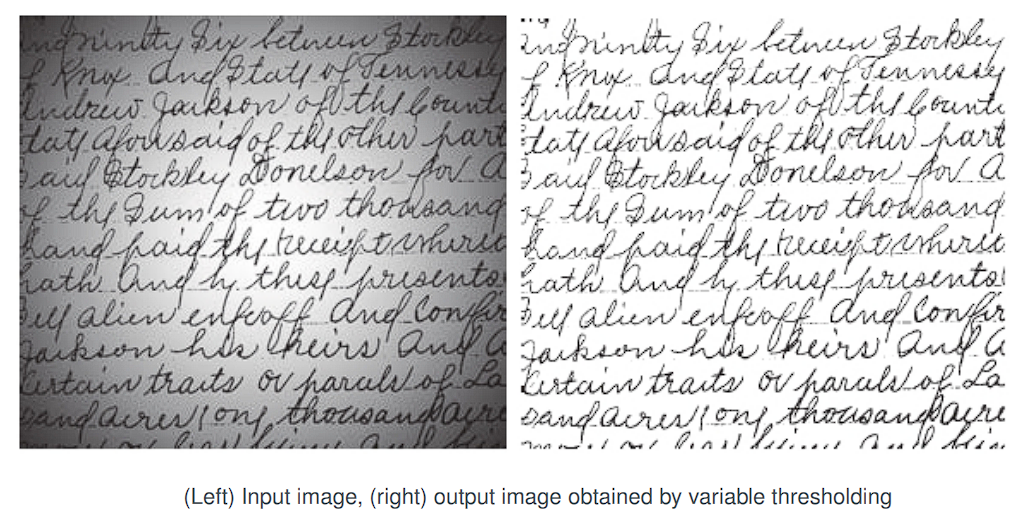
• Scene: Handwritten text corrupted by spot shading (e.g., flash illumination).
• Global Otsu thresholding fails due to strong nonuniform illumination.
• Moving-average local thresholding succeeds:
  • Rule of thumb: set window length n ≈ 5 × average stroke width.
  • Given stroke width ≈ 4 px → choose n = 20.
  • Use c = 0.5.

---

Region Segmentation

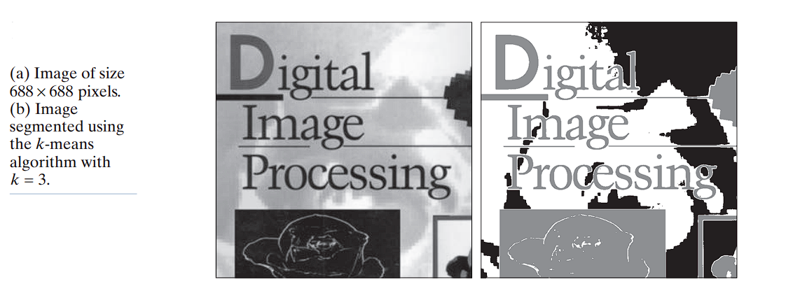
Using K-Means Clustering

The basic idea behind the clustering approach is to partition a set, $Q$, of observations into a specified number, $k$, of clusters. In k-means clustering, each observation is assigned to the cluster with the nearest mean (hence the name of the method), and each mean is called the prototype of its cluster. A k-means algorithm is an iterative procedure that successively refines the means until convergence is achieved.

Let $\{z_1,z_2,\dots ,z_Q\}$ be a set of vector observations (samples). These vectors have the form:

$$z=\left[\begin{array}{c}{z}_1\\ z_2\\ ⋮\\ z_n\end{array}\right]$$

In image segmentation, each component of a vector $z$ represents a numerical pixel attribute. For example:

• If segmentation is based on grayscale intensity, then $z$ is a scalar representing pixel intensity.
• If we are segmenting RGB color images, $z$ is typically a 3-D vector, with each component representing the intensity of a pixel in one of the three primary color channels.

The objective of k-means clustering is to partition the set $Q$ of observations into $k$ disjoint cluster sets:

$$C=\{C_1,C_2,\dots ,C_k\},|C|\le |Q|$$

such that the following criterion of optimality is satisfied:

$$\arg \underset{C_i}{\min }\sum _{i=1}^k\sum _{z\in C_i}\Vert z-m_i{\Vert }^2$$

where $m_i$ is the mean vector (centroid) of the samples in set $C_i$, and $\Vert \arg \Vert$ is the vector norm (typically Euclidean).

In words: we seek the partition such that the sum of squared distances from each point in a cluster to its mean is minimized.

Unfortunately, finding the global minimum is an NP-hard problem, so heuristic methods are used to approximate the solution. Below is the standard k-means algorithm based on the Euclidean distance.

---

Standard K-Means Algorithm

Given a set $\{z_1,z_2,\dots ,z_Q\}$ of vector observations and a specified $k$:

1. Initialization
   Specify an initial set of means:

   $$\{m_1^{(0)},m_2^{(0)},\dots ,m_k^{(0)}\}$$

2. Assign Samples to Clusters
   For each sample $z_q$, assign it to the cluster whose mean is closest:

   $$z_q\in C_i\text{if}\Vert z_q-m_i{\Vert }^2<\Vert z_q-m_j{\Vert }^2,\forall j\ne i$$

3. Update Cluster Centers (Means)
   For each cluster $C_i$:

   $$m_i=\frac{1}{|C_i|}\sum _{z\in C_i}z$$

4. Test for Convergence
   Compute the residual error:

   $$E=\sum _{i=1}^k\Vert m_i^{(t)}-m_i^{(t-1)}\Vert$$

   Stop if $E\le T$, where $T$ is a specified nonnegative threshold; otherwise, return to Step 2.

---

Convergence and Practical Notes

• If $T=0$, the algorithm converges in a finite number of iterations, but only to a local minimum.
• The result depends on the initial choice of means $\{m_i\}$.
• A common practice in data analysis is to choose initial means as $k$ random samples from the dataset and run the algorithm multiple times with different initializations to test stability.
• In image segmentation, however, the most critical issue is the choice of $k$, since it directly determines the number of segmented regions. Therefore, multiple random initializations are less commonly used in this context.

---

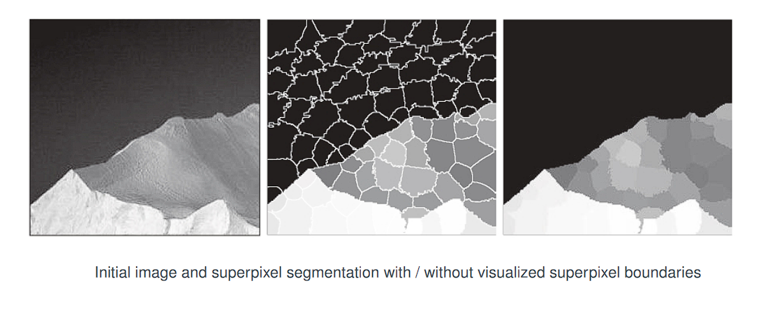
Region Segmentation Using Superpixels

The idea behind superpixels is to replace the standard pixel grid by grouping pixels into primitive regions that are more perceptually meaningful than individual pixels.

• In sensitive applications (e.g., computerized medical diagnosis), approximate representations are often unacceptable.
• However, in domains such as image-database queries, autonomous navigation, and robotics, the benefits of efficiency and improved segmentation performance outweigh the loss of detail.

Primary Requirement: Adherence to Boundaries

One important requirement of any superpixel representation is adherence to boundaries. This means that boundaries between regions of interest must be preserved in a superpixel image.

Effect of Reducing Superpixel Count

The impact of decreasing the number of superpixels is shown

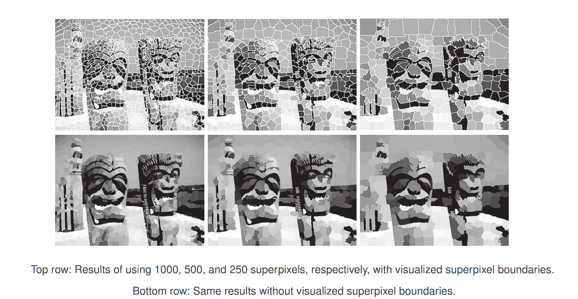
• 1,000 superpixels:

  • Some detail is lost, but most key structures remain visible.

• 500 superpixels:

  • More noticeable loss of detail.
  • Two of the three small carvings on the fence disappear.

• 250 superpixels:

  • The third carving is also lost.
  • Significant simplification occurs, but:
    • The main boundaries remain preserved.
    • The basic topology of the scene is still intact.

---

SLIC Superpixel Algorithm

SLIC is essentially a modification of the k-means clustering algorithm. The difference lies in the definition of the feature space and the distance metric used.

Simple Linear Iterative Clustering (SLIC) generates superpixels by clustering pixels in a joint color–spatial feature space using a variant of k-means. It is conceptually simple and computationally efficient because assignment is restricted to a local window around each cluster center.

---

Representation of Observations

SLIC typically uses (but is not limited to) 5-dimensional vectors containing three color components and two spatial coordinates. For an image in the RGB color space, the vector representation of a pixel is:

z = [ r, g, b, x, y ]ᵀ

where:

• $(r,g,b)$ are the three color components of the pixel.
• $(x,y)$ are the spatial coordinates of the pixel.

---

Initialization

• Let $n_{sp}$ denote the desired number of superpixels.
• Let $n_{tp}$ denote the total number of pixels in the image.

The grid spacing interval $s$ is chosen as:

$$s=\sqrt{\frac{n_{tp}}{n_{sp}}}$$

This ensures that the generated superpixels are approximately equal in area.

The initial superpixel centers are sampled on a regular grid, each represented as:

$$m_i=[r_i,g_i,b_i,x_i,y_i{]}^T,i=1,2,\dots ,n_{sp}$$

To avoid centering a superpixel on an edge or noisy pixel, each initial center is moved to the lowest gradient position in its $3\times 3$ neighborhood.

---

Algorithm Steps

Step 1 — Initialization

• Assign each pixel $p$ a label $L(p)=-1$ and a distance $d(p)=\infty$.
• Place initial cluster centers $m_i$ on a regular grid spaced $s$ units apart.

---

Step 2 — Assignment

• For each cluster center $m_i$, compute the distance $D(p,i)$ between $m_i$ and each pixel $p$ in its local $2s\times 2s$ neighborhood.
• If $D(p,i)<d(p)$, then update: $$d(p)=D(p,i),L(p)=i$$

---

Step 3 — Update

• For each cluster $C_i$, update the cluster center as the mean of all pixels assigned to it:

$$m_i=\frac{1}{|C_i|}\sum _{z\in C_i}z$$

where $|C_i|$ is the number of pixels in cluster $C_i$, and $z$.

---

Step 4 — Convergence Test

• Compute the residual error $E$ as the sum of Euclidean norms of the differences between the new and old cluster centers.
• If $E<T$, where $T$ is a nonnegative threshold, stop. Otherwise, return to Step 2.

---

Step 5 — Post-Processing

• Each superpixel region $C_i$ is assigned a constant value, typically the average of its member pixels:

$$m_i=\frac{1}{|C_i|}\sum _{z\in C_i}z$$

• For grayscale images, this reduces to the average intensity within the superpixel.

SLIC superpixels are formed as clusters in a joint space of color and spatial variables. It is not appropriate to use a single Euclidean distance in this case, since the scales of the color and spatial components are different and unrelated. To address this, SLIC normalizes the distances of the different components and then combines them into a composite distance measure.

Color and Spatial Distances

Let $d_c$ and $d_s$ denote the color and spatial Euclidean distances, respectively, between two points $i$ and $j$ in a cluster.

Color distance:

$$d_c=\sqrt{(r_j-r_i{)}^2+(g_j-g_i{)}^2+(b_j-b_i{)}^2}$$

where $(r,g,b)$ are the pixel color components.

Spatial distance:

$$d_s=\sqrt{(x_j-x_i{)}^2+(y_j-y_i{)}^2}$$

where $(x,y)$ are the pixel coordinates.

---

Composite Distance

The overall distance $D$ is defined as:

$$D=\sqrt{{\left(\frac{d_c}{d_{cm}}\right)}^2+{\left(\frac{d_s}{d_{sm}}\right)}^2}$$

where:

• $d_{cm}$ = maximum expected color distance.
• $d_{sm}$ = maximum expected spatial distance.

The maximum spatial distance is chosen as the sampling interval:

$$d_{sm}=s=\sqrt{\frac{n_{tp}}{n_{sp}}}$$

Determining $d_{cm}$ is more complex, as color variation depends on the cluster and the image. A common approach is to set:

$$d_{cm}=c$$

which transforms Eq into:

$$D=\sqrt{{\left(\frac{d_c}{c}\right)}^2+{\left(\frac{d_s}{s}\right)}^2}$$

or equivalently:

$$D=\sqrt{d_c^2+{\left(\frac{d_s}{s}c\right)}^2}$$

---

• When $c$ is large:

  • Spatial proximity dominates.
  • Superpixels are more compact and uniform.

• When $c$ is small:

  • Color similarity dominates.
  • Superpixels adhere more tightly to object boundaries, but have irregular shapes.

---

Special Cases

• Grayscale images:

  Replace $d_c$ with intensity difference:

  $$d_c=|l_j-l_i|$$

  where $l$ is the pixel intensity.

• 3-D data (supervoxels):

  The spatial distance extends to include the third spatial coordinate $z$:

  $$d_s=\sqrt{(x_j-x_i{)}^2+(y_j-y_i{)}^2+(z_j-z_i{)}^2}$$

  and the feature vector becomes:

  $$z=[r,g,b,x,y,z{]}^T$$

---

SLIC does not inherently enforce connectivity. Thus, after convergence, some isolated pixels may remain. These are reassigned using a connected components algorithm.

---

Notes

• Unlike standard k-means, the SLIC algorithm does not compute distances for all pixels in the image, but rather restricts them to a $2s\times 2s$ neighborhood around each cluster center. This greatly reduces computational cost.
• The distance metric $D(p,i)$ used in SLIC is not purely Euclidean but includes both color and spatial proximity.
• In practice, SLIC convergence can be achieved with relatively large thresholds, e.g., $T=10$ (as reported by Achanta et al., 2012).

SLIC chooses initial centers regularly spaced so that each cluster covers approximately the same number of pixels (voxels, in 3D)

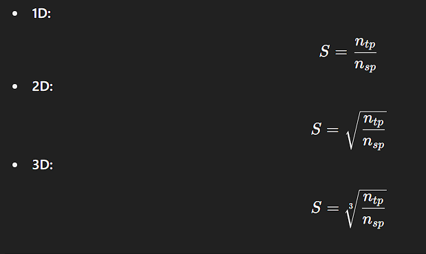
The parameter $S$ in the SLIC algorithm controls the grid spacing for initializing superpixel centers, and thus determines the expected size of a superpixel. Its interpretation differs between 2D images and 1D signals.

In 2D (Standard SLIC): S is the grid spacing for initializing the superpixel centers.

The "size" of a superpixel is its area, which is roughly S x S = S².

Therefore, the relationship is:
(Area per superpixel) * (Number of superpixels) ≈ (Total area)

S² * n_sp ≈ n_tp

S = sqrt(n_tp / n_sp)

In 1D signals, each superpixel is just an interval of length 𝑆.

In one-dimensional signals:

• The notion of “area” reduces to length.
• Each superpixel corresponds to a contiguous interval of the signal.
• Let $S_{\text{len}}$ be the average length of a superpixel.

Then:

$$\text{Length per superpixel}\cdot n_{sp}\approx \text{Total length}$$

or equivalently:

$$S_{\text{len}}\cdot n_{sp}\approx n_{tp}$$

which simplifies to:

$$S_{\text{len}}=\frac{n_{tp}}{n_{sp}}$$

---